Free-free axial rod — natural frequencies

Companion to Fixed-free axial rod — natural frequencies (fixed-free). A uniform rod with both ends free vibrates longitudinally with cosine mode shapes \(u_n(x) = \cos(n \pi x / L)\) and the canonical free-free natural frequencies

\[f_n = \frac{n}{2 L} \sqrt{\frac{E}{\rho}}, \qquad n = 1, 2, 3, \ldots\]

The mode at \(n = 0\) is the rigid-body axial translation — a zero-eigenvalue mode produced by the unconstrained boundary condition. Every elastic frequency \(f_n, n \ge 1\) follows the formula above.

Implementation

Drives the existing FreeFreeRodModes problem class on a 40-element TRUSS2 mesh — the cleanest 1D discretisation of the axial-wave operator (TRUSS2 — 2-node 3D axial bar). Transverse DOFs at every node are pinned to UY = UZ = 0 so the element’s zero transverse stiffness doesn’t admit arbitrary side-sway modes; the axial DOF is unconstrained at both ends, producing the rigid-body / elastic spectrum the closed form predicts.

The extraction filter walks the spectrum starting at 1 Hz to skip the (analytically) zero-frequency rigid-body mode that the solver returns at machine-precision noise level.

References

• Rao, S. S. (2017) Mechanical Vibrations, 6th ed., Pearson, §8.2 Table 8.1 (axial wave equation eigenvalues).

• Meirovitch, L. (2010) Fundamentals of Vibrations, Long Grove, §6.6 (free-free rod).

• Cook, R. D., Malkus, D. S., Plesha, M. E., Witt, R. J. (2002) Concepts and Applications of Finite Element Analysis, 4th ed., Wiley, §11 (modal analysis with rigid-body modes).

Vendor cross-references

Source	Reported f_1 [Hz]	Problem ID / location
Closed form (wave equation)	2 523.77	Rao 2017 §8.2 Table 8.1
Meirovitch (2010) §6.6	2 523.77	free-free rod
MAPDL Verification Manual	≈ 2 524	VM-47 (free-free torsion analogue)
Abaqus Verification Manual	≈ 2 524	AVM 1.6.x free-free rod NF family

from __future__ import annotations

import numpy as np
import pyvista as pv

from femorph_solver.validation.problems import FreeFreeRodModes

Build the model from the validation problem class

problem = FreeFreeRodModes()
m = problem.build_model()
print(
    f"free-free rod mesh: {m.grid.n_points} nodes, {m.grid.n_cells} TRUSS2 cells; "
    f"L = {problem.L} m, E = {problem.E / 1e9:.0f} GPa, ρ = {problem.rho:.1f} kg/m³"
)

c = np.sqrt(problem.E / problem.rho)
f1_published = c / (2.0 * problem.L)
f2_published = 2.0 * f1_published
print()
print(f"Wave speed c = √(E/ρ)        = {c:.3f} m/s")
print(f"f_1 = c / (2 L) (published)  = {f1_published:.3f} Hz")
print(f"f_2 = 2 f_1     (published)  = {f2_published:.3f} Hz")

free-free rod mesh: 41 nodes, 40 TRUSS2 cells; L = 1.0 m, E = 200 GPa, ρ = 7850.0 kg/m³

Wave speed c = √(E/ρ)        = 5047.545 m/s
f_1 = c / (2 L) (published)  = 2523.772 Hz
f_2 = 2 f_1     (published)  = 5047.545 Hz

Modal solve + frequency extraction

A free-free rod exhibits one rigid-body axial-translation mode at \(f = 0\) (machine-precision noise after numeric discretisation). problem.extract skips it via a 1 Hz floor; the next two finite frequencies are the analytical \(f_1, f_2\).

res = m.solve_modal(n_modes=problem.default_n_modes if hasattr(problem, "default_n_modes") else 6)
freqs = np.asarray(res.frequency, dtype=np.float64)

print()
print("  All recovered frequencies (lowest first):")
for k, f in enumerate(freqs):
    label = "rigid-body" if f < 1.0 else "elastic"
    print(f"    mode {k + 1}: f = {f:>10.4f} Hz   ({label})")

f1_computed = problem.extract(m, res, "f1_axial")
f2_computed = problem.extract(m, res, "f2_axial")
err1 = (f1_computed - f1_published) / f1_published * 100.0
err2 = (f2_computed - f2_published) / f2_published * 100.0
print()
print(
    f"  f_1 computed = {f1_computed:.3f} Hz   published = {f1_published:.3f} Hz   err = {err1:+.4f} %"
)
print(
    f"  f_2 computed = {f2_computed:.3f} Hz   published = {f2_published:.3f} Hz   err = {err2:+.4f} %"
)

assert abs(err1) < 2.0, f"f_1 deviation {err1:.3f}% exceeds 2 %"
assert abs(err2) < 5.0, f"f_2 deviation {err2:.3f}% exceeds 5 %"

All recovered frequencies (lowest first):
  mode 1: f =     0.0013 Hz   (rigid-body)
  mode 2: f =  2524.4210 Hz   (elastic)
  mode 3: f =  5052.7355 Hz   (elastic)
  mode 4: f =  7588.8428 Hz   (elastic)

f_1 computed = 2524.421 Hz   published = 2523.772 Hz   err = +0.0257 %
f_2 computed = 5052.736 Hz   published = 5047.545 Hz   err = +0.1028 %

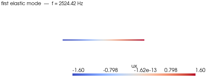
Render the first elastic axial mode

The first elastic mode has \(u(x) = \cos(\pi x / L)\) — antisymmetric about the rod’s midspan, with the two ends moving in opposite directions and a node (zero-displacement) at \(x = L/2\).

shapes = np.asarray(res.mode_shapes).reshape(-1, 3, len(freqs))
elastic_idx = next((k for k, f in enumerate(freqs) if f > 1.0), 0)
phi = shapes[:, :, elastic_idx]

scale = 0.05 * problem.L / max(np.abs(phi).max(), 1e-30)
warped = m.grid.copy()
warped.points = m.grid.points + scale * phi
warped["|phi|"] = np.linalg.norm(phi, axis=1)
warped["ux"] = phi[:, 0]

plotter = pv.Plotter(off_screen=True, window_size=(720, 280))
plotter.add_mesh(m.grid, style="wireframe", color="grey", opacity=0.3)
plotter.add_mesh(warped, scalars="ux", cmap="coolwarm", line_width=4, show_edges=False)
plotter.add_text(
    f"first elastic mode  —  f = {freqs[elastic_idx]:.2f} Hz",
    position="upper_left",
    font_size=11,
)
plotter.view_xy()
plotter.camera.zoom(1.05)
plotter.show()