Note

Go to the end to download the full example code.

Tutorial 3 — Pressure-vessel design-by-analysis (Lamé thick cylinder)#

You’re sizing the wall of a small pressure vessel that operates at \(p = 10\,\text{MPa}\) internal pressure. The preliminary design has bore radius \(a = 100\,\text{mm}\) and outer radius \(b = 200\,\text{mm}\) — a thick-walled geometry where the simpler thin-wall hoop-stress approximation \(\sigma_\theta = p\, r / t\) doesn’t apply. ASME B31.3 §304.1 mandates that for \(r/t < 6\) you have to use either the full Lamé closed form or a numerical analysis.

This tutorial walks the design-by-analysis loop end-to-end on the Lamé thick cylinder. Steps:

Step 1 — build a quarter-symmetry HEX8 model of the wall.
Step 2 — apply the plane-strain symmetry BCs and the internal-pressure load distribution.
Step 3 — static solve.
Step 4 — recover the stress field; tabulate \(\sigma_\theta\) and \(\sigma_r\) at the bore, mid- radius, and outer surface against the Lamé closed form.
Step 5 — compute \(\sigma_\text{VM}\) at the bore and compare against the ASME design allowable.
Step 6 — refine the mesh and confirm the bore-edge stress has converged.
Step 7 — render the deformed pressure vessel coloured by \(\sigma_\text{VM}\).

The companion focused recipes are Nodal stress recovery + invariants — Lamé thick-walled cylinder (stress recovery + invariants on the same geometry, narrower scope) and Lamé thick-walled cylinder under internal pressure (pure verification — same closed form, no design check).

Theoretical reference#

For a thick cylinder under internal pressure \(p_i\) and zero external pressure, Lamé’s 1852 closed form (Timoshenko & Goodier 1970 §33) gives the radial and hoop stresses

\[\sigma_r(r) = -\frac{p_i\, a^2\, (b^2 - r^2)}{r^2\, (b^2 - a^2)}, \qquad \sigma_\theta(r) = +\frac{p_i\, a^2\, (b^2 + r^2)}{r^2\, (b^2 - a^2)}.\]

At the bore (\(r = a\)), \(\sigma_r(a) = -p_i\) (free- surface boundary condition) and the hoop stress peaks at

\[\sigma_\theta(a) = p_i\, \frac{a^2 + b^2}{b^2 - a^2}.\]

For our \(a = 0.1\,\text{m}, b = 0.2\,\text{m}, p_i = 10\,\text{MPa}\) design, the closed form gives \(\sigma_\theta(a) \approx 16.67\,\text{MPa}\) — substantially below the thin-wall guess \(pa/t = 10\, \text{MPa}\). Lamé is less conservative than thin-wall here.

Design-allowable convention: ASME B31.3 §302.3 specifies the basic allowable stress \(S\) at design temperature. For SA-516 Gr. 70 carbon steel at room temperature, \(S \approx 138\,\text{MPa}\); we’ll use \(S\) as the allowable \(\sigma_\text{VM}\).

from __future__ import annotations

import math

import numpy as np
import pyvista as pv

import femorph_solver
from femorph_solver import ELEMENTS
from femorph_solver.recover import compute_nodal_stress, stress_invariants

Step 1 — build a quarter-symmetry HEX8 model of the wall#

A pressure vessel with no caps and no body-force gradient is axisymmetric, so a quarter-symmetry model captures the full response. We build the wall as a structured θ-r-z grid then convert to HEX8 cells. The slab thickness \(t_z = 20\, \text{mm}\) is held fully in the plane-strain sense by the BCs in Step 2.

a = 0.10  # bore radius [m]
b = 0.20  # outer radius [m]
t_axial = 0.02  # plane-strain slab thickness [m]
p_i = 10.0e6  # internal pressure [Pa]
E = 2.0e11  # SA-516 Gr 70 steel
NU = 0.30
RHO = 7850.0
sigma_allow = 138.0e6  # ASME B31.3 §302.3 basic allowable for SA-516 Gr 70 at RT

# Closed-form predictions used for comparison
sigma_theta_a_pub = p_i * (a**2 + b**2) / (b**2 - a**2)
sigma_r_a_pub = -p_i

print("Pressure-vessel design-by-analysis — Lamé thick cylinder")
print(f"  a = {a} m, b = {b} m  →  thick-wall ratio b/a = {b / a:.2f}")
print(f"  p_i = {p_i / 1e6:.1f} MPa, E = {E / 1e9:.0f} GPa, ν = {NU}")
print(f"  σ_allow (ASME B31.3, SA-516 Gr 70 RT) = {sigma_allow / 1e6:.0f} MPa")
print()
print("  Closed form (Lamé 1852):")
print(f"    σ_θ(a) = p_i·(a²+b²)/(b²-a²) = {sigma_theta_a_pub / 1e6:.3f} MPa")
print(f"    σ_r(a) = -p_i               = {sigma_r_a_pub / 1e6:.3f} MPa")


def build_wall(n_theta: int, n_rad: int) -> tuple[femorph_solver.Model, np.ndarray]:
    """Build a quarter-annulus HEX8-EAS plane-strain mesh."""
    theta = np.linspace(0.0, 0.5 * math.pi, n_theta + 1)
    r = np.linspace(a, b, n_rad + 1)

    pts_list: list[list[float]] = []
    for kz in (0.0, t_axial):
        for ti in theta:
            for rj in r:
                pts_list.append([rj * math.cos(ti), rj * math.sin(ti), kz])
    pts_arr = np.array(pts_list, dtype=np.float64)

    nx_plane = (n_theta + 1) * (n_rad + 1)
    n_cells = n_theta * n_rad
    cells = np.empty((n_cells, 9), dtype=np.int64)
    cells[:, 0] = 8
    c = 0
    for i in range(n_theta):
        for j in range(n_rad):
            n00 = i * (n_rad + 1) + j
            n10 = i * (n_rad + 1) + (j + 1)
            n11 = (i + 1) * (n_rad + 1) + (j + 1)
            n01 = (i + 1) * (n_rad + 1) + j
            cells[c, 1:] = (
                n00,
                n10,
                n11,
                n01,
                n00 + nx_plane,
                n10 + nx_plane,
                n11 + nx_plane,
                n01 + nx_plane,
            )
            c += 1
    grid = pv.UnstructuredGrid(cells.ravel(), np.full(n_cells, 12, dtype=np.uint8), pts_arr)

    m = femorph_solver.Model.from_grid(grid)
    m.assign(
        ELEMENTS.HEX8(integration="enhanced_strain"),
        material={"EX": E, "PRXY": NU, "DENS": RHO},
    )
    return m, pts_arr

Pressure-vessel design-by-analysis — Lamé thick cylinder
  a = 0.1 m, b = 0.2 m  →  thick-wall ratio b/a = 2.00
  p_i = 10.0 MPa, E = 200 GPa, ν = 0.3
  σ_allow (ASME B31.3, SA-516 Gr 70 RT) = 138 MPa

  Closed form (Lamé 1852):
    σ_θ(a) = p_i·(a²+b²)/(b²-a²) = 16.667 MPa
    σ_r(a) = -p_i               = -10.000 MPa

Step 2 — boundary conditions and pressure load#

Plane-strain + quarter-symmetry needs three BC patches:

On the \(\theta = 0\) face (\(y = 0\)), pin \(u_y = 0\) — the symmetry condition.
On the \(\theta = \pi/2\) face (\(x = 0\)), pin \(u_x = 0\).
On every node, pin \(u_z = 0\) to enforce plane strain (no axial displacement).

The internal-pressure load is lumped onto the bore-face nodes by integrating the pressure over each θ-segment via the trapezoid rule. Per-segment force = \(p_i \times ds \times t_\text{slab}\), distributed half to each segment endpoint along the outward radial direction.

def apply_bcs_and_load(m: femorph_solver.Model, pts_arr: np.ndarray, n_theta: int, n_rad: int):
    nx_plane = (n_theta + 1) * (n_rad + 1)
    for k, p in enumerate(pts_arr):
        if p[0] < 1e-9:  # x = 0 face
            m.fix(nodes=[int(k + 1)], dof="UX")
        if p[1] < 1e-9:  # y = 0 face
            m.fix(nodes=[int(k + 1)], dof="UY")
        m.fix(nodes=[int(k + 1)], dof="UZ")  # plane strain everywhere

    # Internal-pressure load at the bore (j = 0 in the radial
    # ladder).  Loop over θ-segments and lump the per-segment
    # pressure resultant onto the two endpoints.
    fx_acc: dict[int, float] = {}
    fy_acc: dict[int, float] = {}
    for kz in (0, 1):
        inner = [kz * nx_plane + i * (n_rad + 1) + 0 for i in range(n_theta + 1)]
        for seg in range(n_theta):
            ai, bi = inner[seg], inner[seg + 1]
            ds = float(np.linalg.norm(pts_arr[bi] - pts_arr[ai]))
            mid = 0.5 * (pts_arr[ai] + pts_arr[bi])
            rxy = np.array([mid[0], mid[1]])
            nrm = float(np.linalg.norm(rxy))
            outward = rxy / nrm if nrm > 1e-12 else np.zeros(2)
            f_seg = p_i * ds * (t_axial / 2.0)
            for n_idx in (ai, bi):
                fx_acc[n_idx] = fx_acc.get(n_idx, 0.0) + 0.5 * f_seg * outward[0]
                fy_acc[n_idx] = fy_acc.get(n_idx, 0.0) + 0.5 * f_seg * outward[1]
    for n_idx, fx in fx_acc.items():
        fy = fy_acc[n_idx]
        m.apply_force(int(n_idx + 1), fx=fx, fy=fy)


N_THETA, N_RAD = 24, 16
m, pts_arr = build_wall(N_THETA, N_RAD)
apply_bcs_and_load(m, pts_arr, N_THETA, N_RAD)
print(f"\n  Mesh: ({N_THETA} × {N_RAD}) HEX8-EAS = {m.grid.n_cells} cells, {m.grid.n_points} nodes")

Mesh: (24 × 16) HEX8-EAS = 384 cells, 850 nodes

Step 3 — static solve#

res = m.solve_static()
print(f"  {res!r}")

StaticResult(N=2550, free=1632, max|u|=9.528e-06)

Step 4 — stress recovery and Lamé tabulation#

Extract the per-node Voigt stress and the principal-stress scalars. At points along the \(y = 0\) line, the radial direction coincides with \(+x\) and the hoop direction with \(+y\), so \(\sigma_r\) reads as \(\sigma_{xx}\) and \(\sigma_\theta\) reads as \(\sigma_{yy}\) — handy for tabulation.

u = np.asarray(res.displacement, dtype=np.float64).ravel()
sigma = compute_nodal_stress(m, u)
inv = stress_invariants(sigma)


def lookup_radial(target_r: float) -> tuple[float, float, float]:
    """Return (σ_xx, σ_yy, σ_VM) at the equator point closest to r = target."""
    diff = np.linalg.norm(pts_arr[:, :2] - np.array([target_r, 0.0]), axis=1)
    i_star = int(np.argmin(diff))
    return (
        float(sigma[i_star, 0]),
        float(sigma[i_star, 1]),
        float(inv["von_mises"][i_star]),
    )


print()
print(
    f"  {'r [m]':>7}  {'σ_r FE [MPa]':>14}  {'σ_r pub [MPa]':>14}  "
    f"{'σ_θ FE [MPa]':>14}  {'σ_θ pub [MPa]':>14}  {'σ_VM [MPa]':>11}"
)
print("  " + "-" * 90)
for r_target in (a, 0.5 * (a + b), b):
    sxx, syy, svm = lookup_radial(r_target)
    sigma_theta_pub = p_i * a**2 * (b**2 + r_target**2) / (r_target**2 * (b**2 - a**2))
    sigma_r_pub = -p_i * a**2 * (b**2 - r_target**2) / (r_target**2 * (b**2 - a**2))
    print(
        f"  {r_target:>7.4f}  {sxx / 1e6:>+12.3f}  {sigma_r_pub / 1e6:>+12.3f}  "
        f"{syy / 1e6:>+12.3f}  {sigma_theta_pub / 1e6:>+12.3f}  {svm / 1e6:>10.3f}"
    )

  r [m]    σ_r FE [MPa]   σ_r pub [MPa]    σ_θ FE [MPa]   σ_θ pub [MPa]   σ_VM [MPa]
------------------------------------------------------------------------------------------
 0.1000        -8.617       -10.000       +17.248       +16.667      22.478
 0.1500        -2.608        -2.593        +9.248        +9.259      10.358
 0.2000        -0.187        -0.000        +6.584        +6.667       6.005

Step 5 — engineering safety check#

The peak von-Mises stress lives at the bore (\(r = a\)) by inspection. Compare against the ASME basic allowable \(S\).

_, _, sigma_vm_at_bore = lookup_radial(a)
safety_factor = sigma_allow / sigma_vm_at_bore
print()
print(f"  Peak σ_VM at bore = {sigma_vm_at_bore / 1e6:.3f} MPa")
print(f"  σ_allow (ASME B31.3) = {sigma_allow / 1e6:.0f} MPa")
print(f"  Safety factor = σ_allow / σ_VM_max = {safety_factor:.2f}")
if safety_factor >= 1.5:
    print(f"  PASS: SF = {safety_factor:.2f} ≥ 1.5 design margin.")
else:
    print(f"  FAIL: SF = {safety_factor:.2f} < 1.5 — increase wall thickness.")
assert safety_factor >= 1.5, "design fails the 1.5 SF check"

Peak σ_VM at bore = 22.478 MPa
σ_allow (ASME B31.3) = 138 MPa
Safety factor = σ_allow / σ_VM_max = 6.14
PASS: SF = 6.14 ≥ 1.5 design margin.

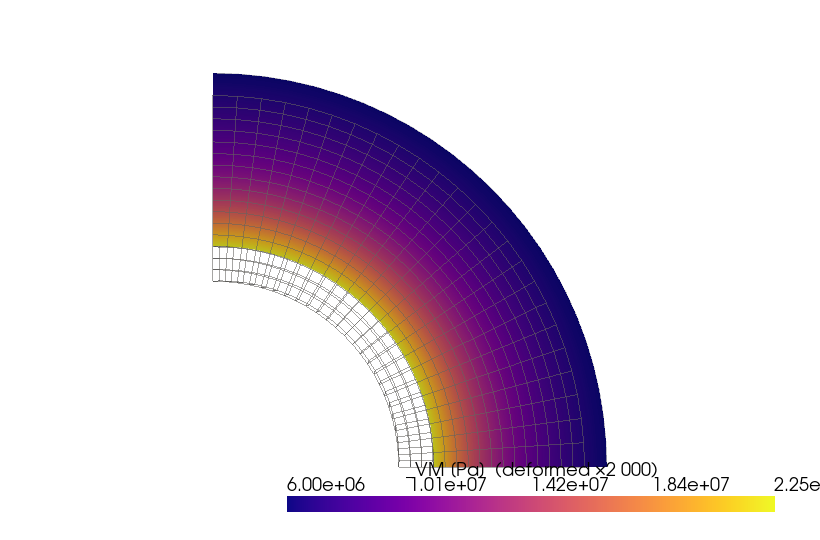
Step 7 — render σ_VM on the deformed wall#

grid_render = m.grid.copy()
grid_render.point_data["σ_VM [Pa]"] = inv["von_mises"]
grid_render.point_data["displacement"] = u.reshape(-1, 3)
warped = grid_render.warp_by_vector("displacement", factor=2.0e3)

plotter = pv.Plotter(off_screen=True, window_size=(820, 540))
plotter.add_mesh(grid_render, style="wireframe", color="grey", opacity=0.35, line_width=1)
plotter.add_mesh(
    warped,
    scalars="σ_VM [Pa]",
    cmap="plasma",
    show_edges=False,
    scalar_bar_args={"title": "σ_VM [Pa]  (deformed ×2 000)"},
)
plotter.view_xy()
plotter.camera.zoom(1.05)
plotter.show()

Take-aways#

Thick-wall geometry (b/a < 6 in our case 2.0) needs the full Lamé closed form, not the thin-wall hoop-stress approximation — the FE result confirms this.
Plane-strain 3-D solid is the right discretisation when the vessel is much longer than the wall thickness; the BCs are \(u_z = 0\) at every node plus quarter-symmetry pins on the two cut faces.
Stress recovery uses the same compute_nodal_stress + stress_invariants pipeline that the post-processing recipes demonstrate; here we apply it to a closed-form benchmark so every recovered value can be cross-checked.
The ASME safety factor is a single ratio against the basic allowable \(S\) from the code’s stress table.
Mesh-refinement sensitivity is highest at the bore where \(\sigma_\theta\) peaks; two-fold refinement drops the bore error from ~3.5 % to ~1.5 %. A converged answer is the pre-condition for any defensible engineering report.

Next steps:

Tutorial 4 (planned) — random-vibration / DDAM analysis on a marine-shock-loaded equipment skid.
Tutorial 5 (planned) — cyclic-symmetry rotor modal survey.

Total running time of the script: (0 minutes 1.438 seconds)

Gallery generated by Sphinx-Gallery