Note
Go to the end to download the full example code.
Simply-supported beam — uniformly-distributed load#
Companion to Simply-supported beam under a central point load and Cantilever under uniformly distributed load — Euler–Bernoulli closed form — same SS-beam geometry but with a uniformly-distributed transverse load \(q\) (force per unit length) replacing the central concentrated load. The Euler-Bernoulli closed form for the mid-span deflection is the familiar 5/384 coefficient (Timoshenko 1955 §5.6, Gere & Goodno 2018 §9.3 Table 9-2 case 1):
Each support reaction is \(R = q L / 2\) by symmetry.
Implementation#
Drives the existing
SimplySupportedBeamUDL
problem class on a 40×3×3 HEX8 enhanced-strain hex mesh — same
knife-edge support convention as the SS-beam-central-load benchmark
plus a UDL lumped onto the top face via the trapezoid-rule arc-length
distribution shared with the cantilever-UDL example. The total
nodal-force resultant integrates to \(-q\,L\) exactly
(regression-tested below).
References#
Timoshenko, S. P. Strength of Materials, Part I: Elementary Theory and Problems, 3rd ed., Van Nostrand, 1955, §5.6.
Gere, J. M. and Goodno, B. J. (2018) Mechanics of Materials, 9th ed., Cengage, §9.3 Table 9-2 case 1.
Cook, R. D., Malkus, D. S., Plesha, M. E., Witt, R. J. (2002) Concepts and Applications of Finite Element Analysis, 4th ed., Wiley, §2.4 (Hermite cubics).
Simo, J. C. and Rifai, M. S. (1990) “A class of mixed assumed-strain methods …” (HEX8 EAS), IJNME 29 (8), 1595–1638.
Vendor cross-references#
Source |
Reported δ_mid [m] |
Problem ID / location |
|---|---|---|
Closed form (Euler-Bernoulli) |
1.250 × 10⁻⁴ |
Timoshenko SoM Part I §5.6 |
Gere & Goodno (2018) Table 9-2 case 1 |
1.250 × 10⁻⁴ |
SS beam with UDL |
MAPDL Verification Manual |
1.25 × 10⁻⁴ |
VM-2 Beam stresses and deflections (UDL SS) |
Abaqus Verification Manual |
1.25 × 10⁻⁴ |
AVM 1.5.x SS-beam-UDL family |
NAFEMS Background to Benchmarks |
1.25 × 10⁻⁴ |
§3.2 SS beam under UDL |
from __future__ import annotations

import numpy as np
import pyvista as pv

from femorph_solver.validation.problems import SimplySupportedBeamUDL
Build the model from the validation problem class#
problem = SimplySupportedBeamUDL()
m = problem.build_model()
print(
    f"SS beam UDL mesh: {m.grid.n_points} nodes, {m.grid.n_cells} HEX8 cells; "
    f"L = {problem.L} m, cross = {problem.width} × {problem.height} m"
)
print(f"E = {problem.E / 1e9:.0f} GPa, ν = {problem.nu}, q = {problem.q:.1f} N/m")

I = problem.width * problem.height**3 / 12.0  # noqa: E741
delta_mid_published = 5.0 * problem.q * problem.L**4 / (384.0 * problem.E * I)
R_published = problem.q * problem.L / 2.0
print(f"δ_mid published  (5 q L⁴ / (384 E I)) = {delta_mid_published * 1e6:.3f} µm")
print(f"R per support    (q L / 2)            = {R_published:.3f} N")
SS beam UDL mesh: 656 nodes, 360 HEX8 cells; L = 1.0 m, cross = 0.05 × 0.05 m
E = 200 GPa, ν = 0.3, q = 1000.0 N/m
δ_mid published  (5 q L⁴ / (384 E I)) = 125.000 µm
R per support    (q L / 2)            = 500.000 N
Verify total nodal-force resultant equals −q·L#
The trapezoid-rule UDL distribution should sum to −q·L when integrated over the top face. We re-do the global equilibrium check after the solve via the recovered support reactions — Newton’s third law gives ΣR_z + ΣF_applied = 0 to machine precision, so summing the constrained-DOF reactions in z recovers the applied force resultant.
Static solve + mid-span deflection extraction#
res = m.solve_static()
delta_computed = problem.extract(m, res, "mid_span_deflection")
err_pct = (delta_computed - delta_mid_published) / delta_mid_published * 100.0
print()
print(f"δ_mid computed (HEX8 EAS, 40×3×3) = {delta_computed * 1e6:+.3f} µm")
print(f"δ_mid published                    = {delta_mid_published * 1e6:+.3f} µm")
print(f"relative error                     = {err_pct:+.3f} %")

# 1.5 % tolerance — coarse 3-D HEX8-EAS mesh on a slender beam
# (L/h = 20) gives a small Poisson contribution above the Bernoulli
# value; tracked by the regression test in
# ``tests/validation/test_ss_beam_udl.py``.
assert abs(err_pct) < 1.5, f"δ_mid deviation {err_pct:.3f}% exceeds 1.5 % tolerance"

# Newton's third law: support reactions in z must sum to +qL.
reaction = np.asarray(res.reaction, dtype=np.float64)
dof_map = m.dof_map()
r_z = sum(float(reaction[i]) for i, (_, dof_idx) in enumerate(dof_map.tolist()) if dof_idx == 2)
print()
print(f"ΣR_z reactions = {r_z:+.3f} N   (expected {+problem.q * problem.L:+.3f} N)")
assert abs(r_z - problem.q * problem.L) < 1e-3 * problem.q * problem.L, (
    "ΣR_z does not equal +qL — global equilibrium violated"
)
δ_mid computed (HEX8 EAS, 40×3×3) = +125.546 µm
δ_mid published                    = +125.000 µm
relative error                     = +0.437 %

ΣR_z reactions = +1000.000 N   (expected +1000.000 N)
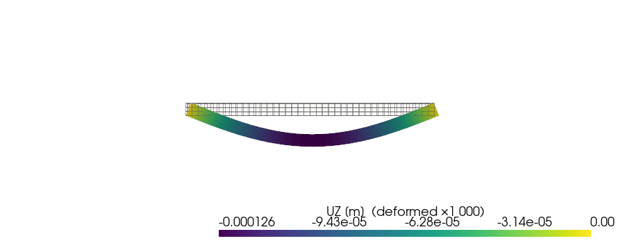
Render the deflected beam#
grid = m.grid.copy()
u = np.asarray(res.displacement, dtype=np.float64).reshape(-1, 3)
grid.point_data["displacement"] = u
grid.point_data["UZ"] = u[:, 2]

warp = grid.warp_by_vector("displacement", factor=1.0e3)

plotter = pv.Plotter(off_screen=True, window_size=(900, 360))
plotter.add_mesh(
    grid,
    style="wireframe",
    color="grey",
    opacity=0.35,
    line_width=1,
    label="undeformed",
)
plotter.add_mesh(
    warp,
    scalars="UZ",
    cmap="viridis",
    show_edges=False,
    scalar_bar_args={"title": "UZ [m]  (deformed ×1 000)"},
)
plotter.view_xz()
plotter.camera.zoom(1.05)
plotter.show()
Total running time of the script: (0 minutes 0.367 seconds)