Tutorial 2 — Modal survey of a cantilever bracket#

Picking up from Tutorial 1 — Cantilever beam under combined loading, the static analysis confirmed the bracket carries its design load with a comfortable safety margin. But the equipment console it supports has variable-speed motors that excite the bracket at multiple harmonics across the operating band. The next question is dynamic: do any of the bracket’s natural frequencies fall inside the excitation band, and if so which modes need to be included in a response-spectrum analysis to capture 90 % of the modal mass?

This tutorial walks the modal-survey workflow end-to-end:

Step 1 — build the same cantilever geometry from Tutorial 1, this time as a 3-D solid that carries its own mass (no separate tip mass, just the bracket’s structural mass distributed by ρ × V).
Step 2 — run a modal solve and inspect the spectrum.
Step 3 — identify each mode’s character (transverse bending, axial, torsional) by inspecting the recovered eigenvectors.
Step 4 — compute modal participation factors and effective modal mass per excitation direction (X, Y, Z).
Step 5 — read the cumulative-effective-mass curve to pick \(n_\text{modes}\) for a response-spectrum analysis meeting the ASCE 7 / Eurocode 8 90 % threshold.
Step 6 — render the lowest few mode shapes for the design-review packet.

The post-processing recipes for participation factors and mode-shape animation live in Modal participation factors + effective modal mass and Mode-shape animation — cantilever bending modes — they exercise the same APIs in narrower scope.

Theoretical reference#

A free-vibration modal analysis solves the generalised symmetric-definite eigenvalue problem (Modal eigenvalue problem and shift-invert Lanczos)

\[\mathbf{K}\, \boldsymbol{\phi}_i = \omega_i^{2}\, \mathbf{M}\, \boldsymbol{\phi}_i,\]

with \(\mathbf{K}\) and \(\mathbf{M}\) the assembled stiffness and mass matrices. Each eigenpair returns one mode shape \(\boldsymbol{\phi}_i\) and one natural frequency \(f_i = \omega_i / (2\pi)\).

For base-excitation analysis (the bracket bolted to a vibrating floor), the modal participation factor for mode \(i\) in direction \(d\) is

\[\Gamma_i^{(d)} = \frac{\boldsymbol{\phi}_i^\top \mathbf{M}\, \mathbf{r}^{(d)}} {\boldsymbol{\phi}_i^\top \mathbf{M}\, \boldsymbol{\phi}_i},\]

where \(\mathbf{r}^{(d)}\) is the influence vector — ones on every translational DOF along direction \(d\), zeros elsewhere. The corresponding effective modal mass is

\[M_\text{eff,i}^{(d)} = (\Gamma_i^{(d)})^{2} \cdot \boldsymbol{\phi}_i^\top \mathbf{M}\, \boldsymbol{\phi}_i,\]

and the partition-of-unity property \(\sum_i M_\text{eff,i}^{(d)} = M_\text{total}\) lets the cumulative effective-mass curve answer the design-code question “how many modes do I need?”.

References: Bathe 2014 §9.3.4, Chopra 2017 §13.1, Cook et al. 2002 §11.6.

from __future__ import annotations

import numpy as np
import pyvista as pv

import femorph_solver
from femorph_solver import ELEMENTS

Step 1 — build the bracket#

Same prismatic-cantilever geometry and material as Tutorial 1, this time at slightly higher slenderness to push the first transverse-bending frequency lower. We keep HEX8-EAS so the bending modes don’t shear-lock.

E = 2.0e11  # Pa, steel
NU = 0.30
RHO = 7850.0  # kg/m³
L = 1.0  # m
WIDTH = 0.05
HEIGHT = 0.05

NX, NY, NZ = 60, 3, 3
xs = np.linspace(0.0, L, NX + 1)
ys = np.linspace(0.0, WIDTH, NY + 1)
zs = np.linspace(0.0, HEIGHT, NZ + 1)
grid = pv.StructuredGrid(*np.meshgrid(xs, ys, zs, indexing="ij")).cast_to_unstructured_grid()

m = femorph_solver.Model.from_grid(grid)
m.assign(
    ELEMENTS.HEX8(integration="enhanced_strain"),
    material={"EX": E, "PRXY": NU, "DENS": RHO},
)

pts = np.asarray(m.grid.points)
node_nums = np.asarray(m.grid.point_data["ansys_node_num"], dtype=np.int64)
clamped = np.where(pts[:, 0] < 1e-9)[0]
m.fix(nodes=node_nums[clamped].tolist(), dof="ALL")

total_mass = RHO * L * WIDTH * HEIGHT
print("Cantilever bracket — modal survey")
print(f"  L = {L} m, cross = {WIDTH} × {HEIGHT} m, ρ = {RHO} kg/m³")
print(f"  Mesh: {NX} × {NY} × {NZ} HEX8-EAS = {m.grid.n_cells} cells, {m.grid.n_points} nodes")
print(f"  Total structural mass M_total = ρ·L·A = {total_mass:.3f} kg")

Cantilever bracket — modal survey
  L = 1.0 m, cross = 0.05 × 0.05 m, ρ = 7850.0 kg/m³
  Mesh: 60 × 3 × 3 HEX8-EAS = 540 cells, 976 nodes
  Total structural mass M_total = ρ·L·A = 19.625 kg

Step 3 — mode-shape character via translation-energy split#

Each mode mixes translational components. A transverse- bending mode has nearly all its kinetic energy in \(u_y\) (or \(u_z\)); an axial mode has it in \(u_x\); a torsional mode has the warping pattern characteristic of Saint-Venant torsion.

We classify each mode by the per-direction translation-energy fraction. The square cross-section makes \(y\) / \(z\) bending pairs degenerate, so transverse modes appear in pairs at the same frequency.

dof_map = m.dof_map()
classifications = []
for i in range(N_MODES):
    phi = shapes[:, i]
    energy_total = (phi**2).sum()
    energy_per_dof = np.zeros(3)
    for row, (_node, dof_idx) in enumerate(dof_map.tolist()):
        if dof_idx < 3:
            energy_per_dof[int(dof_idx)] += phi[row] ** 2
    fractions = energy_per_dof / (energy_total + 1e-30)
    # Pick the dominant direction.
    label = ("axial (x)", "transverse-y", "transverse-z")[int(np.argmax(fractions))]
    classifications.append((label, fractions))

print()
print(f"  {'mode':>4}  {'f [Hz]':>9}  {'character':>14}  {'%U_x':>6}  {'%U_y':>6}  {'%U_z':>6}")
print("  " + "-" * 53)
for i, (label, frac) in enumerate(classifications):
    print(
        f"  {i + 1:>4}  {freqs[i]:>9.3f}  {label:>14}  "
        f"{100 * frac[0]:>5.1f}%  {100 * frac[1]:>5.1f}%  {100 * frac[2]:>5.1f}%"
    )

mode     f [Hz]       character    %U_x    %U_y    %U_z
-----------------------------------------------------
   40.831    transverse-z    0.2%    0.8%   99.0%
   40.831    transverse-y    0.2%   99.0%    0.8%
  253.268    transverse-y    1.1%   75.9%   23.0%
  253.268    transverse-z    1.1%   23.0%   75.9%
  698.142    transverse-z    2.4%   38.2%   59.4%
  698.142    transverse-y    2.4%   59.4%   38.2%
  750.821    transverse-z    0.0%   50.0%   50.0%
 1264.431       axial (x)  100.0%    0.0%    0.0%
 1338.909    transverse-z    4.2%   23.7%   72.1%
 1338.909    transverse-y    4.2%   72.1%   23.7%
 2156.450    transverse-z    6.1%   35.0%   58.9%
 2156.450    transverse-y    6.1%   58.9%   35.0%

Step 5 — design-code mode-count threshold#

ASCE 7 §12.9 and Eurocode 8 §4.3.3.3 both require at least 90 % cumulative effective mass in every direction the response-spectrum input acts. Read the thresholds off the cumulative table.

target_pct = 90.0
for d_idx, dname in enumerate(("X", "Y", "Z")):
    crossings = np.where(cum_pct[:, d_idx] >= target_pct)[0]
    if len(crossings) > 0:
        n_required = int(crossings[0]) + 1
        print(
            f"  {dname}: needs ≥ {n_required} modes for {target_pct:.0f} % cumulative effective mass "
            f"({cum_pct[n_required - 1, d_idx]:.2f} % at mode {n_required})"
        )
    else:
        print(
            f"  {dname}: {N_MODES} modes only reach {cum_pct[-1, d_idx]:.2f} % — "
            f"needs more modes to clear {target_pct:.0f} % threshold"
        )

# X direction has no bending modes in the first 12 (all bending
# is transverse y / z), so X stays at 0 % cumulative mass — that's
# the correct physics for a slender cantilever where axial modes
# only appear far above the bending fundamentals.  Asserts only
# Y / Z which are the design-relevant directions.
y_n = (
    int(np.where(cum_pct[:, 1] >= target_pct)[0][0]) + 1
    if (cum_pct[:, 1] >= target_pct).any()
    else N_MODES
)
z_n = (
    int(np.where(cum_pct[:, 2] >= target_pct)[0][0]) + 1
    if (cum_pct[:, 2] >= target_pct).any()
    else N_MODES
)
n_for_response_spectrum = max(y_n, z_n)
print()
print(
    f"  → Use n_modes = {n_for_response_spectrum} for a 3-direction "
    f"response-spectrum analysis (max over Y / Z; X is axial-only and "
    f"out of the bending band the equipment excites)."
)
assert n_for_response_spectrum <= N_MODES, "default 12 modes was too few — increase the solve"

X: 12 modes only reach 80.89 % — needs more modes to clear 90 % threshold
Y: needs ≥ 10 modes for 90 % cumulative effective mass (90.06 % at mode 10)
Z: needs ≥ 10 modes for 90 % cumulative effective mass (90.06 % at mode 10)

→ Use n_modes = 10 for a 3-direction response-spectrum analysis (max over Y / Z; X is axial-only and out of the bending band the equipment excites).

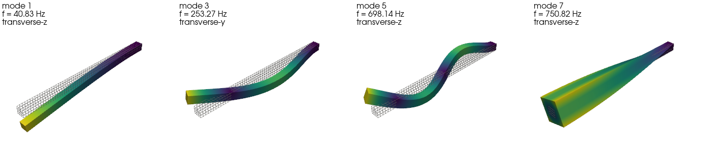
Step 6 — render the lowest four mode shapes#

mode_pairs = []
seen_freqs: list[float] = []
for i in range(N_MODES):
    f = freqs[i]
    if any(abs(f - sf) < 1e-3 for sf in seen_freqs):
        continue
    seen_freqs.append(float(f))
    mode_pairs.append(i)
    if len(mode_pairs) >= 4:
        break

plotter = pv.Plotter(shape=(1, 4), off_screen=True, window_size=(1400, 320), border=False)
for col, idx in enumerate(mode_pairs):
    plotter.subplot(0, col)
    grid_warped = m.grid.copy()
    n_pts = grid_warped.n_points
    disp = np.zeros((n_pts, 3))
    for row, (node, dof_idx) in enumerate(dof_map.tolist()):
        if dof_idx < 3:
            pt_idx = np.where(node_nums == int(node))[0]
            if len(pt_idx):
                disp[pt_idx[0], int(dof_idx)] += shapes[row, idx]
    peak = float(np.linalg.norm(disp, axis=1).max())
    scale = 0.10 * L / peak if peak > 0 else 1.0
    grid_warped.points = np.asarray(m.grid.points) + scale * disp
    grid_warped["|disp|"] = np.linalg.norm(disp, axis=1)
    plotter.add_mesh(m.grid, style="wireframe", color="grey", opacity=0.3)
    plotter.add_mesh(
        grid_warped,
        scalars="|disp|",
        cmap="viridis",
        show_edges=False,
        show_scalar_bar=False,
    )
    plotter.add_text(
        f"mode {idx + 1}\nf = {freqs[idx]:.2f} Hz\n{classifications[idx][0]}",
        position="upper_left",
        font_size=9,
    )
    plotter.view_isometric()
    plotter.camera.zoom(1.05)
plotter.link_views()
plotter.show()

Take-aways#

The modal solve is a single Model.solve_modal(n_modes=N) call; the eigensolver picks shift-invert Lanczos automatically (Modal analysis).
Mode classification by translation-energy fraction is a robust filter against degenerate transverse pairs and stray torsional modes — works on any geometry.
Modal participation + effective mass is computed from first principles via Model.mass_matrix() plus the per-direction influence vector built from Model.dof_map().
Mode-count selection for response-spectrum analysis reads directly off the cumulative-effective-mass table: ASCE 7 / Eurocode 8 require ≥ 90 % per direction.
Mode-shape rendering uses the same scatter pattern as Plotting mode shapes — display amplitude is scaled to a fraction of the bounding box (mode shapes carry no absolute magnitude).

Next steps:

Tutorial 3 (planned) — pressure-vessel design-by-analysis on a Lamé thick cylinder.
For a worked response-spectrum computation that builds on this modal survey, see the planned Tutorial 4 — it convolves a synthetic ASCE 7 design spectrum with the participation-factor table generated above.

Total running time of the script: (0 minutes 1.636 seconds)

Gallery generated by Sphinx-Gallery