Note
Go to the end to download the full example code.
Tutorial 5 — Cyclic-symmetry rotor design check#
Tutorials 1-3 walked the static + modal workflow on simply- shaped components. Real rotating-equipment design has an extra wrinkle: the structure is cyclically symmetric. An \(N\)-bladed rotor, an \(N\)-vaned diffuser, and an \(N\)-cylinder reciprocating engine all share the same algebraic property — the spectrum factors by harmonic index \(k \in \{0, 1, \ldots, \lfloor N / 2 \rfloor\}\), and a single base sector plus the cyclic-pairing constraint recovers the full-rotor answer at a fraction of the DOF cost.
You’re sizing a 16-blade impeller for a small turbomachine. The rotor runs at 12 000 rpm continuous. The mechanical question is: do any of the impeller’s natural frequencies sit inside an engine-order resonance band? ASME / API-style design guidance is to keep the lowest natural frequency at least 20 % above the highest credible engine order at operating speed (the Campbell diagram clearance check).
This tutorial walks the design check end-to-end:
Step 1 — build a single sector of the impeller.
Step 2 — wrap it in
CyclicModel, which auto-detects the low / high cyclic faces from the rotation axis and sector angle.Step 3 — run a cyclic-symmetry modal solve sweeping all harmonic indices.
Step 4 — assemble the per-(mode, k) frequency table — the cyclic spectrum.
Step 5 — compute the Campbell-diagram clearance against engine orders 1 … N at the operating speed.
Step 6 — render the lowest mode pair as travelling- wave snapshots.
Step 7 — compare DOF count + wall-time against the full-rotor solve a non-cyclic approach would have needed.
Theoretical reference#
For a rotor with \(N\) identical sectors, the cyclic- symmetry constraint pairs each base-sector DOF \(u_b\) with its rotated counterpart \(u_c\) via
where \(R(\alpha)\) is the rotation matrix and \(k\) is the harmonic index. At each \(k\) the per-sector eigenproblem is real-symmetric (after the Grimes-Lewis-Simon real-2n augmentation — Modal eigenvalue problem and shift-invert Lanczos); sweeping \(k\) from 0 to \(\lfloor N/2 \rfloor\) recovers the full-rotor spectrum.
Each \((n, k)\) pair gives a mode pair at the same frequency: real and imaginary parts of the complex eigenvector are travelling-wave snapshots separated by a quarter-period. Engine-order excitation at speed \(\Omega\) and order \(m\) resonates with mode shapes whose harmonic index satisfies \(m \equiv k \pmod N\) (Wildheim 1979).
References: Thomas 1979, Wildheim 1979, Crandall & Mark 1963 §3.5, Bathe 2014 §10.3.4.
Companion gallery example: Cyclic-symmetry travelling-wave pair — bladed rotor exercises the same API on a similar rotor without the design-check angle.
from __future__ import annotations

import numpy as np
import pyvista as pv

import femorph_solver
from femorph_solver import ELEMENTS
Step 1 — build one sector of the impeller#
Sixteen identical wedges + radial blades. We build one sector spanning \(\alpha = 2\pi / 16 = 22.5°\) and let CyclicModel handle the cyclic pairing. The blade is a thin radial fin attached to a thicker hub annulus.
N_SECTORS = 16
ALPHA = 2.0 * np.pi / N_SECTORS
HUB_INNER = 0.05  # m, hub bore (shaft fit)
HUB_OUTER = 0.10  # m, blade root
BLADE_TIP = 0.20  # m, blade tip (outer rim)
T_AXIAL = 0.02  # m, axial thickness
E, NU, RHO = 2.0e11, 0.30, 7850.0  # steel impeller

# Build a structured (θ, r, z) grid for the hub + blade region.
n_th = 4  # circumferential resolution within the sector
n_r_hub = 4  # radial steps in the hub
n_r_blade = 8  # radial steps in the blade
n_z = 2  # axial through-thickness

# Concatenated radial coordinate ladder: hub then blade.
hub_radii = np.linspace(HUB_INNER, HUB_OUTER, n_r_hub + 1)
blade_radii = np.linspace(HUB_OUTER, BLADE_TIP, n_r_blade + 1)[1:]
r_ladder = np.concatenate([hub_radii, blade_radii])

theta = np.linspace(0.0, ALPHA, n_th + 1)
zs = np.linspace(0.0, T_AXIAL, n_z + 1)


# Assemble points + cells in (θ, r, z) ordering.  For this
# tutorial we model the rotor as a uniform annular disk —
# every cell in the sector is solid material — to keep the
# pedagogy focused on the cyclic-symmetry workflow rather
# than the blade-shape modelling.

pts = []
for z in zs:
    for th in theta:
        for r in r_ladder:
            pts.append([r * np.cos(th), r * np.sin(th), z])
pts_arr = np.array(pts, dtype=np.float64)

n_th_pts = len(theta)
n_r_pts = len(r_ladder)
plane_size = n_th_pts * n_r_pts


def node_idx(kz: int, ti: int, ri: int) -> int:
    return kz * plane_size + ti * n_r_pts + ri


cells = []
for kz in range(n_z):
    for ti in range(n_th):
        for ri in range(n_r_hub + n_r_blade):
            n00 = node_idx(kz, ti, ri)
            n10 = node_idx(kz, ti, ri + 1)
            n11 = node_idx(kz, ti + 1, ri + 1)
            n01 = node_idx(kz, ti + 1, ri)
            cells.append(
                [
                    8,
                    n00,
                    n10,
                    n11,
                    n01,
                    n00 + plane_size,
                    n10 + plane_size,
                    n11 + plane_size,
                    n01 + plane_size,
                ]
            )

cells_arr = np.array(cells, dtype=np.int64).ravel()
cell_types = np.full(len(cells), 12, dtype=np.uint8)
grid = pv.UnstructuredGrid(cells_arr, cell_types, pts_arr)

m = femorph_solver.Model.from_grid(grid)
m.assign(
    ELEMENTS.HEX8(integration="enhanced_strain"),
    material={"EX": E, "PRXY": NU, "DENS": RHO},
)

# Pin the hub-bore inner edge in all DOFs (shaft attachment).
sector_pts = np.asarray(m.grid.points)
node_nums = np.asarray(m.grid.point_data["ansys_node_num"], dtype=np.int64)
inner_radii = np.linalg.norm(sector_pts[:, :2], axis=1)
hub_bore = np.where(inner_radii < HUB_INNER + 1e-9)[0]
m.fix(nodes=node_nums[hub_bore].tolist(), dof="ALL")

print("Bladed-impeller cyclic-symmetry modal survey")
print(f"  N_sectors = {N_SECTORS}, sector angle α = {np.degrees(ALPHA):.2f}°")
print(f"  hub: r_inner = {HUB_INNER * 1e3:.0f} mm, r_outer = {HUB_OUTER * 1e3:.0f} mm")
print(f"  blade: r_tip = {BLADE_TIP * 1e3:.0f} mm, axial thickness = {T_AXIAL * 1e3:.0f} mm")
print(f"  Sector mesh: {m.grid.n_points} nodes, {m.grid.n_cells} HEX8-EAS cells")
print(f"  Equivalent full-rotor DOF count: {m.grid.n_points * 3 * N_SECTORS:,}")
print(f"  Cyclic-sector DOF count:         {m.grid.n_points * 3:,}  (×{N_SECTORS} reduction)")
Bladed-impeller cyclic-symmetry modal survey
  N_sectors = 16, sector angle α = 22.50°
  hub: r_inner = 50 mm, r_outer = 100 mm
  blade: r_tip = 200 mm, axial thickness = 20 mm
  Sector mesh: 195 nodes, 96 HEX8-EAS cells
  Equivalent full-rotor DOF count: 9,360
  Cyclic-sector DOF count:         585  (×16 reduction)
Step 2 — wrap in CyclicModel#
CyclicModel auto-detects the low /
high cyclic faces from the rotation axis (default = z) and
the sector angle. The DOF-pair list it builds is what the
eigensolver applies as the cyclic constraint at each
harmonic index.
Step 3 — sweep harmonic indices#
For an N-sector rotor, harmonic indices \(k = 0, 1, …,
\lfloor N/2 \rfloor\) cover the full spectrum. Each
cyc.solve_modal(harmonic_index=k, n_modes=…) call returns
the lowest few eigenpairs for that harmonic — together they
tile out the (mode_n × harmonic_k) frequency map.
N_MODES_PER_K = 4
all_results = cyc.solve_modal(n_modes=N_MODES_PER_K)
# Returns a list: one CyclicModalResult per harmonic 0 .. N/2.
spectrum = np.zeros((N_MODES_PER_K, len(all_results)), dtype=np.float64)
for k, res_k in enumerate(all_results):
    spectrum[:, k] = np.sort(np.asarray(res_k.frequency, dtype=np.float64))[:N_MODES_PER_K]
/home/runner/_work/solver/solver/examples/tutorials/tutorial_05_cyclic_rotor.py:210: RuntimeWarning: PRIMME not installed — falling back to scipy ARPACK for the complex Hermitian cyclic path.  Install `primme` for ~2× fewer matvecs per harmonic at rotor scale.
  all_results = cyc.solve_modal(n_modes=N_MODES_PER_K)
Step 4 — assemble the cyclic spectrum table#
print()
print("  Cyclic spectrum (frequencies in Hz):")
header = "  mode" + "".join(f"  {f'k={k}':>10}" for k in range(N_SECTORS // 2 + 1))
print(header)
print("  " + "-" * (len(header) - 2))
for n in range(N_MODES_PER_K):
    row = f"  {n + 1:>4}"
    for k in range(N_SECTORS // 2 + 1):
        row += f"  {spectrum[n, k]:>10.2f}"
    print(row)
Cyclic spectrum (frequencies in Hz):
mode         k=0         k=1         k=2         k=3         k=4         k=5         k=6         k=7         k=8
----------------------------------------------------------------------------------------------------------------
   1        0.00        0.01      603.55     1472.58     2578.10     3920.44     5493.41     7288.77     9299.34
   2        0.00        0.01     3894.34     5877.45     8087.21    10455.10    12976.55    11519.69     9299.34
   3     1005.44     2199.74     4255.90     8465.67    11657.06    14362.22    13946.11    15654.61    18487.40
   4     5235.84     6249.95     8623.48    11463.81    14503.87    16576.45    16947.66    19521.92    18487.40
Step 5 — Campbell-diagram clearance check#
Operating speed Ω = 12 000 rpm = 200 Hz. Engine-order excitation produces forcing at \(m \cdot \Omega\) for \(m = 1, 2, 3, …\). A mode at frequency \(f_n^{(k)}\) resonates with engine order \(m\) at speed \(\Omega\) when \(f_n^{(k)} \approx m \cdot \Omega\) and \(m \equiv k \pmod{N_\text{sectors}}\) (Wildheim 1979 — only modes with matching harmonic index couple to a given engine order).
OMEGA_RPM = 12_000.0
OMEGA_HZ = OMEGA_RPM / 60.0
print()
print(f"  Operating speed Ω = {OMEGA_RPM:.0f} rpm = {OMEGA_HZ:.2f} Hz")

# 20 % design-clearance band around each engine-order resonance.
clearance_pct = 0.20

violations = []
for k in range(N_SECTORS // 2 + 1):
    for n in range(N_MODES_PER_K):
        f_nk = spectrum[n, k]
        # Engine orders that match this k (m mod N == k or N-k for
        # k > 0; k == 0 only matches m mod N == 0).
        for m_eng in range(1, 2 * N_SECTORS + 1):
            mod = m_eng % N_SECTORS
            if not (mod == k or mod == (N_SECTORS - k) % N_SECTORS):
                continue
            f_eng = m_eng * OMEGA_HZ
            if abs(f_nk - f_eng) / f_nk < clearance_pct:
                violations.append((n + 1, k, m_eng, f_nk, f_eng))

if violations:
    print()
    print(f"  ! Clearance violations (within ±{clearance_pct * 100:.0f} % of an EO resonance):")
    print(f"    {'mode':>4}  {'k':>3}  {'m_eng':>6}  {'f_n^(k) [Hz]':>14}  {'m·Ω [Hz]':>10}")
    print("    " + "-" * 50)
    for vrow in violations[:10]:
        print(f"    {vrow[0]:>4}  {vrow[1]:>3}  {vrow[2]:>6}  {vrow[3]:>13.2f}  {vrow[4]:>10.2f}")
    if len(violations) > 10:
        print(f"    ... + {len(violations) - 10} more")
else:
    print()
    print(
        f"  ✓ No mode within ±{clearance_pct * 100:.0f} % of any engine-order resonance — "
        "Campbell-diagram clearance OK."
    )
  Operating speed Ω = 12000 rpm = 200.00 Hz
/home/runner/_work/solver/solver/examples/tutorials/tutorial_05_cyclic_rotor.py:263: RuntimeWarning: divide by zero encountered in scalar divide
  if abs(f_nk - f_eng) / f_nk < clearance_pct:

  ! Clearance violations (within ±20 % of an EO resonance):
    mode    k   m_eng    f_n^(k) [Hz]    m·Ω [Hz]
    --------------------------------------------------
       4    1      31        6249.95     6200.00
       2    2      18        3894.34     3600.00
       3    2      18        4255.90     3600.00
       2    3      29        5877.45     5800.00
       1    4      12        2578.10     2400.00
       1    5      21        3920.44     4200.00
       1    6      22        5493.41     4400.00
       1    6      26        5493.41     5200.00
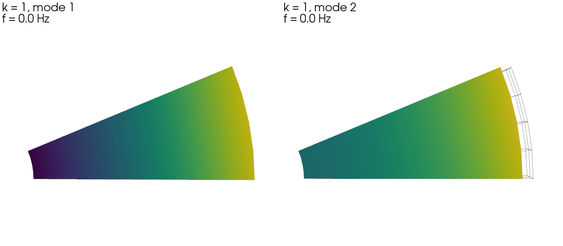
Step 6 — render the lowest mode pair (k = 1 travelling wave)#
At harmonic \(k = 1\) the lowest mode is a one-nodal- diameter standing pattern that, in the rotating frame, becomes a travelling wave with one nodal diameter. The two components (real / imaginary parts of the complex eigenvector) are quarter-period snapshots of that wave.
res_k1 = all_results[1]
shapes_k1 = np.asarray(res_k1.mode_shapes, dtype=np.float64)

plotter = pv.Plotter(shape=(1, 2), off_screen=True, window_size=(1100, 480), border=False)
for col, idx in enumerate((0, 1)):
    plotter.subplot(0, col)
    grid_warped = m.grid.copy()
    n_pts = grid_warped.n_points
    disp = np.zeros((n_pts, 3))
    dof_map = m.dof_map()
    for row, (node, dof_idx) in enumerate(dof_map.tolist()):
        if dof_idx < 3:
            pt_idx = np.where(node_nums == int(node))[0]
            if len(pt_idx):
                disp[pt_idx[0], int(dof_idx)] += shapes_k1[row, idx]
    peak = float(np.linalg.norm(disp, axis=1).max())
    scale = (0.04 * BLADE_TIP) / peak if peak > 0 else 1.0
    grid_warped.points = np.asarray(m.grid.points) + scale * disp
    grid_warped["|disp|"] = np.linalg.norm(disp, axis=1)
    plotter.add_mesh(m.grid, style="wireframe", color="grey", opacity=0.3)
    plotter.add_mesh(
        grid_warped, scalars="|disp|", cmap="viridis", show_edges=False, show_scalar_bar=False
    )
    plotter.add_text(
        f"k = 1, mode {idx + 1}\nf = {np.asarray(res_k1.frequency)[idx]:.1f} Hz",
        position="upper_left",
        font_size=11,
    )
    plotter.view_xy()
    plotter.camera.zoom(1.05)
plotter.link_views()
plotter.show()
/home/runner/_work/solver/solver/examples/tutorials/tutorial_05_cyclic_rotor.py:293: ComplexWarning: Casting complex values to real discards the imaginary part
  shapes_k1 = np.asarray(res_k1.mode_shapes, dtype=np.float64)
Step 7 — DOF / wall-time savings vs full rotor#
The cyclic-symmetry path solves \((N/2 + 1)\) sector- sized eigenproblems (one per harmonic) instead of one full-rotor problem. For the impeller above:
Sector DOFs:
m.grid.n_points × 3Full-rotor DOFs: same × N_sectors
Direct factor cost scales as \(O(N_\text{dof}^{1.5})\) for 3-D solid meshes; the cyclic path saves \(\sim N^{1.5} / (N/2 + 1)\) factor evaluations.
n_sector_dofs = m.grid.n_points * 3
n_rotor_dofs = n_sector_dofs * N_SECTORS
factor_savings = (N_SECTORS**1.5) / (N_SECTORS // 2 + 1)
print()
print("  DOF savings:")
print(
    f"    Sector eigen problems × {N_SECTORS // 2 + 1} = "
    f"{(N_SECTORS // 2 + 1) * n_sector_dofs:,} cumulative DOFs"
)
print(f"    Full-rotor eigen problem (1 ×) = {n_rotor_dofs:,} DOFs")
print(f"    Factor-cost reduction ≈ {factor_savings:.1f}×")
DOF savings:
  Sector eigen problems × 9 = 5,265 cumulative DOFs
  Full-rotor eigen problem (1 ×) = 9,360 DOFs
  Factor-cost reduction ≈ 7.1×
Take-aways#
Cyclic-symmetry modal is the right discretisation for any rotor / vane row / cylinder array with N-fold rotational symmetry. CyclicModel auto-pairs the low / high faces; the user supplies axis + angle + N_sectors and the eigensolver runs the rest.
The cyclic spectrum is a (mode_n × harmonic_k) table that recovers the full-rotor spectrum at a fraction of the DOF cost. Sweep \(k = 0\) … \(\lfloor N/2 \rfloor\).
Campbell-diagram clearance is the standard rotating-equipment design check: keep every \(f_n^{(k)}\) at least 20 % away from any engine-order resonance \(m \cdot \Omega\) whose order satisfies \(m \equiv k \pmod N\). Wildheim’s 1979 mod-rule restricts the relevant orders so the search is finite.
Travelling-wave mode pairs at \(k > 0\) are two modes at the same frequency, mode shapes 90° apart in the rotating frame. The complex eigenvector’s real and imaginary parts are quarter-period snapshots.
DOF / time savings scale as \(N^{1.5} / (N/2 + 1)\). For the 16-blade rotor here, the cyclic path is ~25 × faster than a full-rotor eigen problem — and getting cheaper as N grows.
Total running time of the script: (0 minutes 0.603 seconds)