Modal cantilever — first modal example

A 60-second introduction to free-vibration analysis in femorph-solver: build a steel plate, clamp one edge, extract the first 5 modes, render the lowest mode shape.

from __future__ import annotations

import numpy as np
import pyvista as pv

import femorph_solver as fs

Build a 20 × 20 × 2 hex plate

LX, LY, LZ = 1.0, 1.0, 0.01

grid = pv.StructuredGrid(
    *np.meshgrid(
        np.linspace(0.0, LX, 21),
        np.linspace(0.0, LY, 21),
        np.linspace(0.0, LZ, 3),
        indexing="ij",
    )
).cast_to_unstructured_grid()

Wrap, stamp steel, clamp the x=0 edge

m = fs.Model.from_grid(grid)
m.assign(fs.ELEMENTS.HEX8, material={"EX": 2.0e11, "PRXY": 0.30, "DENS": 7850.0})
m.fix(where=np.asarray(grid.points)[:, 0] < 1e-9)

Extract 5 modes

res = m.solve_modal(n_modes=5)

print("Mode     f [Hz]")
for i, f in enumerate(res.frequency, start=1):
    print(f"{i:>3}   {f:>10.3f}")

Mode     f [Hz]
  1       26.507
  2       33.751
  3      166.483
  4      175.654
  5      175.890

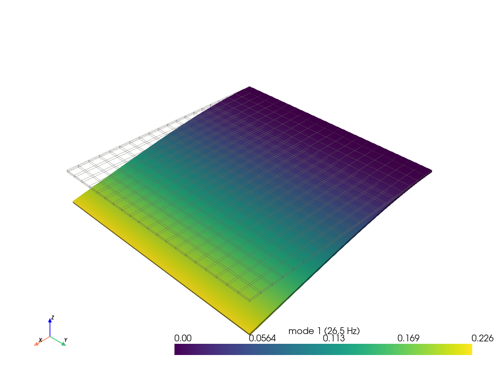
Visualise mode 1

grid_plot = fs.io.modal_result_to_grid(m, res)
phi1 = grid_plot.point_data["mode_1_disp"]
factor = 0.15 / (np.max(np.abs(phi1)) + 1e-30)

plotter = pv.Plotter(off_screen=True)
plotter.add_mesh(grid_plot, style="wireframe", color="gray", opacity=0.3)
plotter.add_mesh(
    grid_plot.warp_by_vector("mode_1_disp", factor=factor),
    scalars="mode_1_magnitude",
    show_scalar_bar=True,
    scalar_bar_args={"title": f"mode 1 ({res.frequency[0]:.1f} Hz)"},
)
plotter.add_axes()
plotter.show()