Note

Go to the end to download the full example code.

Tutorial 6 — End-to-end deliverable workflow#

The earlier tutorials all built their meshes natively in pyvista. Real engineering workflows rarely start that way: the geometry comes out of a CAD tool through a meshing pre-processor (HyperMesh, ANSA, Gmsh) and lands as a deck — almost always an MAPDL CDB or a NASTRAN BDF — that the analyst hands off to the solver, plus a snapshot of the solver-ready model that downstream consumers re-load.

This tutorial walks the complete deliverable workflow from a pre-built model snapshot through a modal-plus-static analysis to a saved .pv result file the analyst can hand the next person on the team. Six steps:

Step 1 — load a model snapshot and inspect what landed. Counts, element types, materials, units, and BCs.
Step 2 — fill in the gaps. Pre-built snapshots sometimes ship without the BC / load setup the next analysis needs; we register them natively.
Step 3 — run a modal solve and read the spectrum.
Step 4 — set up a static load case from scratch on top of the snapshot’s geometry, solve it, and recover the stress field.
Step 5 — save the static result to a self-contained .pv file and re-load it through the disk-backed StaticResultDisk handle.
Step 6 — render a stress-distribution histogram for the design-review packet.

This is the canonical end-to-end workflow the docs missed before — every other gallery example focuses on one slice (reader, solver, recovery, plotting). Tutorial 6 stitches them all together.

Note on the source format#

The tutorial uses the bundled femorph_solver.examples.cyclic_bladed_rotor_sector_path() .pv fixture as the input. The same workflow applies when the source is an MAPDL CDB / NASTRAN BDF / Abaqus INP — call femorph_solver.interop.mapdl.from_cdb() / from_bdf() / from_inp() instead of Model.from_pv() in Step 1, and the rest is identical.

Companion deeper-dive resources#

MAPDL interop — full MAPDL compatibility deep-dive (KEYOPT parity, binary-file coverage).
NASTRAN migration, Abaqus migration — equivalent migration deep-dives for the other two vendor decks.
Result objects — how the disk-backed result handles work.
Static analysis, Modal analysis — the analysis-type pages each step exercises.

from __future__ import annotations

import tempfile
from pathlib import Path

import matplotlib

matplotlib.use("Agg")  # headless: no GUI window pop in gallery / CI

import matplotlib.pyplot as plt
import numpy as np

import femorph_solver
from femorph_solver.recover import compute_nodal_stress, stress_invariants
from femorph_solver.result.static import StaticResultDisk

Step 1 — load the model snapshot#

The bundled cyclic_bladed_rotor_sector_path returns a .pv file that is a complete Model.save() snapshot of one sector of a bladed-rotor disk meshed with HEX8 cells. Real workflows would point Model.from_pv() at the engineer’s own .pv (or call the relevant vendor-deck reader from femorph_solver.interop); the API call is the same.

Model.from_pv returns a native Model carrying everything stamped on the snapshot: geometry, connectivity, element-type registry, materials, real-constant table, the UnitSystem stamp, and any BCs / loads the snapshot author registered. No re-parsing — the .pv is the canonical Model on-disk format.

source_path = femorph_solver.examples.cyclic_bladed_rotor_sector_path()
print(f"Loading model snapshot:\n  {source_path}\n")

model = femorph_solver.Model.from_pv(source_path)

print("After load:")
print(f"  Nodes:                  {model.n_nodes}")
print(f"  Elements:               {model.n_elements}")
print(f"  Element-type registry:  {model.etypes}")
print(f"  Materials:              {list(model.materials.keys())}")
print(f"  Unit-system stamp:      {model.unit_system}")

Loading model snapshot:
  /home/runner/_work/solver/solver/src/femorph_solver/examples/_data/cyclic_bladed_rotor_sector.pv

After load:
  Nodes:                  230
  Elements:               101
  Element-type registry:  {185: 'HEX8'}
  Materials:              [1]
  Unit-system stamp:      UnitSystem.UNSPECIFIED

Step 2 — fill in the gaps#

Looking at the load-time inspection: the snapshot declared one element type and one material. That’s typical — many pre-built models ship with the geometry + materials but without the BC setup the next analysis needs (because BCs are analysis-specific, not model-specific). We register them natively.

This step uses the same Model.fix and Model.apply_force calls every other tutorial uses — the foreign-deck-loader contract is “after the loader returns, the resulting Model is indistinguishable from one built natively”.

pts = np.asarray(model.grid.points)
node_nums = np.asarray(model.grid.point_data["ansys_node_num"], dtype=np.int64)

z_min = pts[:, 2].min()
hub_mask = pts[:, 2] < z_min + 1e-6
print(f"\n  Hub face at z={z_min:.4f} carries {int(hub_mask.sum())} nodes.")

model.fix(nodes=node_nums[hub_mask].tolist(), dof="ALL")
print("  Clamped the hub face (full-fix).")

Hub face at z=-0.7875 carries 10 nodes.
Clamped the hub face (full-fix).

Step 4 — static load case + stress recovery#

Static analysis on the same model. We push a 1000 N axial load distributed across the tip face, solve, recover the stress field, and read out the peak von Mises.

Note that the solve reuses the BCs already on the model from Step 2 — the cyclic faces of the sector are not fixed (that’s appropriate for a fully-tip-loaded static demo). Real cyclic-symmetry analysis would use CyclicModel and its solve_modal(); this tutorial keeps the static case simple to focus on the workflow.

z_max = pts[:, 2].max()
tip_mask = pts[:, 2] > z_max - 1e-6
tip_nodes = node_nums[tip_mask]
TOTAL_LOAD = 1000.0  # arbitrary, in the snapshot's unit system

per_node = TOTAL_LOAD / tip_nodes.size
for n in tip_nodes:
    model.apply_force(int(n), fz=per_node)
print(f"\n  Applied {TOTAL_LOAD} units total across {tip_nodes.size} tip nodes.")

static = model.solve_static()
print(f"  Static solve done.  displacement.shape = {static.displacement.shape}")

# Stress recovery via the public free-function helper.  Same
# math as `StaticResultDisk.stress(model=model)` after the result
# is loaded from disk (Step 5); we use the in-memory path here
# because the model is already in scope.
displacement = static.displacement.reshape(-1, 3)  # 3 DOFs / node
print(f"  Peak displacement magnitude: {np.linalg.norm(displacement, axis=1).max():.4e}")

stress_field = compute_nodal_stress(model, static.displacement)
invariants = stress_invariants(stress_field)
sigma_vm = invariants["von_mises"]
peak_vm = float(sigma_vm.max())
print(f"  Peak von Mises stress: {peak_vm:.3e}")

Applied 1000.0 units total across 5 tip nodes.
Static solve done.  displacement.shape = (690,)
Peak displacement magnitude: 1.5792e-01
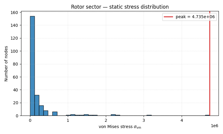
Peak von Mises stress: 4.735e+06

Step 5 — save / reload through the disk-backed StaticResultDisk#

The in-memory result lives in RAM only; the disk-backed StaticResultDisk is the format you hand to the next person on the team. .save writes a single self-contained .pv (zstd-compressed pyvista) file; StaticResultDisk(path) re-loads it lazily.

We write to tempfile.TemporaryDirectory so the gallery build doesn’t litter the source tree, but real workflows would write to a project-results directory and check the .pv into the deliverables folder.

with tempfile.TemporaryDirectory() as tmp:
    out = static.save(Path(tmp) / "rotor_sector_static.pv", model)
    print(f"\n  Wrote: {out.name}  ({out.stat().st_size / 1024:.1f} KiB)")

    # Re-load through the disk-backed handle.  Lazy IO — the
    # full grid only inflates on first .grid access.
    handle = StaticResultDisk(out)
    print(f"  Re-loaded: {type(handle).__name__} from {out.name}")
    print(f"  Disk-backed n_points: {handle.n_points}")

    # Stress recovery on the disk-backed handle uses the same
    # call shape as the in-memory path; the model has to be in
    # scope because stress isn't stored on disk (see
    # /reference/theory/stress_recovery).
    stress_handle = handle.stress(model=model)
    np.testing.assert_allclose(stress_handle, stress_field)
    print("  Round-tripped stress field matches the in-memory recovery.")

    # The lazy disk-backed handle is the canonical way to keep
    # several large analyses in scope without burning RAM.
    print(f"  Available point arrays: {sorted(handle.available_point_arrays())}")

Wrote: rotor_sector_static.pv  (18.3 KiB)
Re-loaded: StaticResultDisk from rotor_sector_static.pv
Disk-backed n_points: 230
Round-tripped stress field matches the in-memory recovery.
Available point arrays: ['REFINE', 'VTKorigID', 'angles', 'ansys_node_num', 'displacement', 'force', 'origid', 'vtkOriginalPointIds']

Step 6 — render the stress histogram#

A simple histogram of the von-Mises field plus a max-line annotation — enough to drop into a design-review slide and read off “where’s the peak and how broad is the distribution?”. Real packets would also include the rendered mesh from Principal stresses + principal directions on a thick cylinder, but this tutorial is about the workflow rather than the final plot polish.

fig, ax = plt.subplots(figsize=(7.5, 4.5))
ax.hist(sigma_vm, bins=40, color="C0", edgecolor="k", alpha=0.85)
ax.axvline(peak_vm, color="C3", lw=2.0, label=f"peak = {peak_vm:.3e}")
ax.set_xlabel(r"von Mises stress $\sigma_\mathrm{vm}$")
ax.set_ylabel("Number of nodes")
ax.set_title("Rotor sector — static stress distribution")
ax.legend(loc="upper right")
ax.grid(True, ls=":", alpha=0.5)
fig.tight_layout()
plt.show()

Rotor sector — static stress distribution

Engineering takeaway#

Three things to read off the workflow before the deliverable:

Snapshot-side gaps are routine. The .pv snapshot came in without analysis-specific BCs / loads — the analyst’s first move was to register them. Any pre-built-model workflow includes a “what did the snapshot declare vs what do I still need to assign” pass; the inspection in Step 1 surfaces it explicitly.
The solver doesn’t care where the mesh came from. Steps 3 and 4 use the same APIs as the from-scratch tutorials. This is the foreign-deck-reader contract: after from_cdb() / from_bdf() / from_inp() / Model.from_pv() returns, the resulting Model is indistinguishable from one built natively.
The .pv result file is the deliverable, not the script. Step 5 round-trips through .pv because that’s how the next person on the team picks the result up. The file carries the displacement + every metadata field, and stress is recovered on demand from the model the consumer has in scope. See Stress recovery from a discrete displacement field for why stress is not stored on disk.

What’s missing (and where to find it):

A composite cross-check against an originating MAPDL run — that’s the verification-corpus pattern in Verification, not what a typical analyst needs in their day-to-day workflow.
A cyclic-symmetry expansion — Tutorial 5 — Cyclic-symmetry rotor design check shows it; the modal solve in Step 3 is the static single-sector form.
A NASTRAN-deck variant — same pattern with femorph_solver.interop.nastran.from_bdf() instead.

Total running time of the script: (0 minutes 1.042 seconds)

Gallery generated by Sphinx-Gallery