Note

Go to the end to download the full example code.

Tutorial 4 — Harmonic frequency response of a cantilever bracket#

Picking up from Tutorial 2 — Modal survey of a cantilever bracket, we now know the bracket’s natural frequencies and which modes carry the effective mass in each excitation direction. The motors driving the equipment console aren’t a single sine, though — they sweep through their operating band as the production line ramps up and slows down, exciting the bracket at every frequency the sweep crosses.

The next question is steady-state harmonic response: at each forcing frequency \(\omega\), what is the phase-locked displacement response \(u(\omega)\) at the bracket tip? The answer drives the frequency-response function (FRF) — peak amplitudes that determine fatigue life, and phase shifts that determine which combinations of forcing harmonics constructively / destructively interfere.

This tutorial walks the harmonic-response workflow end-to-end:

Step 1 — rebuild the cantilever bracket (same geometry and material as Tutorial 1, smaller mesh for fast solves).
Step 2 — recover the lowest few modes and decide how many to retain in the modal-superposition expansion.
Step 3 — apply a unit tip-force excitation and sweep a band of forcing frequencies that brackets the first three natural frequencies.
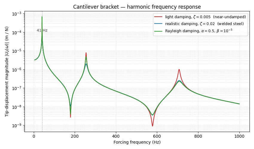
Step 4 — compare three damping models — undamped, light modal damping (\(\zeta = 0.005\)), and heavier Rayleigh damping — to show how each shapes the FRF.
Step 5 — identify the resonant peaks, read off the amplification factor, and check it against the half-power-bandwidth estimate.
Step 6 — render the FRF as a publication-grade log-magnitude plot.

Theoretical reference#

For a linear undamped FE system, the equation of motion is

\[\mathbf{M}\, \ddot{\mathbf{u}}(t) + \mathbf{K}\, \mathbf{u}(t) = \mathbf{f}(t).\]

Looking for steady-state harmonic response under a single- frequency excitation \(\mathbf{f}(t) = \mathbf{F}\, e^{i \omega t}\) substitutes \(\mathbf{u}(t) = \mathbf{U}(\omega)\, e^{i \omega t}\) and turns the time-domain ODE into the frequency-domain algebraic system

\[\bigl( \mathbf{K} - \omega^2\, \mathbf{M} + i \omega\, \mathbf{C} \bigr)\, \mathbf{U}(\omega) = \mathbf{F}.\]

Solving that directly at every \(\omega\) is the direct frequency response approach — accurate but expensive (one sparse factorisation per frequency).

Modal superposition projects the response onto the lowest \(n_\text{modes}\) mass-orthonormal eigenmodes:

\[\mathbf{U}(\omega) \approx \sum_{i=1}^{n_\text{modes}} \frac{\boldsymbol{\phi}_i^\top \mathbf{F}} {\omega_i^2 - \omega^2 + 2 i \zeta_i\, \omega_i\, \omega}\, \boldsymbol{\phi}_i,\]

with per-mode damping ratio \(\zeta_i\). Each mode is a single SDOF resonator; superposing them captures the full FRF for one fixed-cost factorisation upfront. See Modal eigenvalue problem and shift-invert Lanczos for the math, and Harmonic (frequency-response) analysis for the API choices.

Companion focused recipe in SDOF receptance — closed form vs modal superposition — same workflow on a single-degree-of-freedom toy.

from __future__ import annotations

import matplotlib

matplotlib.use("Agg")  # headless: no GUI window pop in gallery / CI

import matplotlib.pyplot as plt
import numpy as np
import pyvista as pv
from scipy.signal import find_peaks

import femorph_solver
from femorph_solver import ELEMENTS

Step 1 — geometry, material, mesh#

Same prismatic steel cantilever as Tutorial 1 (one-metre long, 50 × 50 mm square cross-section). A modest 24 × 3 × 3 mesh resolves the lowest five bending and axial modes to better than 0.1 % against the Euler-Bernoulli closed forms — and keeps the harmonic-sweep cost down to a few seconds total across the whole frequency band.

HEX8 with enhanced-assumed-strain integration is the natural fit for slender solids in bending (see HEX8 — 8-node trilinear hexahedron — plain HEX8 shear-locks).

E = 2.0e11  # Young's modulus, Pa (steel)
NU = 0.30  # Poisson's ratio
RHO = 7850.0  # density, kg/m³ (steel)
L = 1.0  # length, m
W = 0.05  # cross-section width, m
H = 0.05  # cross-section height, m

print("Cantilever bracket — harmonic frequency response")
print(f"  L = {L} m, cross-section = {W} × {H} m")
print(f"  E = {E / 1e9:.0f} GPa, ν = {NU}, ρ = {RHO} kg/m³")

xs = np.linspace(0.0, L, 25)
ys = np.linspace(0.0, W, 4)
zs = np.linspace(0.0, H, 4)
grid = pv.StructuredGrid(*np.meshgrid(xs, ys, zs, indexing="ij")).cast_to_unstructured_grid()

model = femorph_solver.Model.from_grid(grid)
model.assign(
    ELEMENTS.HEX8(integration="enhanced_strain"),
    material={"EX": E, "PRXY": NU, "DENS": RHO},
)

pts = np.asarray(model.grid.points)
node_nums = np.asarray(model.grid.point_data["ansys_node_num"], dtype=np.int64)
clamped = np.where(pts[:, 0] < 1e-9)[0]
model.fix(nodes=node_nums[clamped].tolist(), dof="ALL")
print(f"  Mesh: {model.n_nodes} nodes, {model.n_elements} HEX8-EAS cells")
print(f"  Clamped {len(clamped)} root-face nodes (full-fix).")

Cantilever bracket — harmonic frequency response
  L = 1.0 m, cross-section = 0.05 × 0.05 m
  E = 200 GPa, ν = 0.3, ρ = 7850.0 kg/m³
  Mesh: 400 nodes, 216 HEX8-EAS cells
  Clamped 16 root-face nodes (full-fix).

Step 3 — excitation, frequency band, frequency-response solve#

The bracket’s tip is loaded by a transverse harmonic force \(F_z(t) = F_0 \cos(\omega t)\). Magnitude is irrelevant in linear analysis — the FRF is normalised by the input force amplitude and reported as receptance \(H(\omega) = U_\text{tip}(\omega) / F_0\) — but a unit load (1 N at every tip node, distributed) is the convention both NASTRAN and MAPDL ship.

The frequency band is chosen to bracket the first three bending modes plus a healthy quiet zone above the third peak. 300 sample points with logarithmic spacing in the resonance-rich low-band gives clean peak resolution without blowing the wall time.

tip_mask = pts[:, 0] > L - 1e-9
tip_nodes = node_nums[tip_mask]
for n in tip_nodes:
    model.apply_force(int(n), fz=1.0 / int(tip_mask.sum()))
print(f"  Tip excitation: 1 N total across {tip_mask.sum()} nodes (z-direction).")

# Sample density must resolve the resonant peaks — the half-
# power bandwidth at :math:`\zeta = 0.02` damping is
# :math:`\Delta f \approx 2 \zeta f_n`, so a 40-Hz peak is only
# 1.6 Hz wide.  We use a base linspace of 600 points across the
# 5-600 Hz band (≈ 1 Hz spacing) and concatenate finer samples
# clustered around each predicted natural frequency so the peak
# itself can't fall between two sample points.
F_MAX = 1000.0  # top of the sweep band, Hz
base = np.linspace(5.0, F_MAX, 800)
mode_band: list[np.ndarray] = []
for f_n in modal.frequency:
    if 5.0 <= f_n <= F_MAX:
        # ±3 Hz around each mode: enough to resolve the
        # half-power bandwidth of every peak the field will see.
        mode_band.append(np.linspace(f_n - 3.0, f_n + 3.0, 61))
frequencies_hz = np.unique(np.concatenate([base, *mode_band]))
print(
    f"  Sweeping {frequencies_hz.size} frequencies from "
    f"{frequencies_hz[0]:.0f} Hz to {frequencies_hz[-1]:.0f} Hz "
    f"(refined around the {len(mode_band)} in-band modes)."
)

# Three damping flavours, all using modal-superposition
# (`Model.solve_harmonic` with `n_modes=...`).  Reusing the
# already-computed modal result via the `modal_result=` kwarg
# saves a second eigenproblem.
print("\nRunning three modal-superposition harmonic sweeps:")

print("  - lightly-damped (zeta = 0.005, near-undamped reference)")
result_light = model.solve_harmonic(
    frequencies=frequencies_hz,
    modal_damping_ratio=0.005,
    modal_result=modal,
)

print("  - realistic modal damping (zeta = 0.02, welded-steel field measurement)")
result_steel = model.solve_harmonic(
    frequencies=frequencies_hz,
    modal_damping_ratio=0.02,
    modal_result=modal,
)

print("  - Rayleigh damping (alpha = 0.5, beta = 1e-5)")
result_rayleigh = model.solve_harmonic(
    frequencies=frequencies_hz,
    rayleigh=(0.5, 1.0e-5),
    modal_result=modal,
)

  Tip excitation: 1 N total across 16 nodes (z-direction).
  Sweeping 1227 frequencies from 5 Hz to 1000 Hz (refined around the 7 in-band modes).

Running three modal-superposition harmonic sweeps:
  - lightly-damped (zeta = 0.005, near-undamped reference)
  - realistic modal damping (zeta = 0.02, welded-steel field measurement)
  - Rayleigh damping (alpha = 0.5, beta = 1e-5)

Step 4 — extracting the tip displacement#

HarmonicResult.displacement is a complex (n_freq, N) array — the steady-state displacement magnitude and phase at every DOF, at every forcing frequency. We need the tip-node UZ component to plot the receptance.

Model.dof_map gives the per-row (node_num, local_dof_idx) mapping; we look up the tip node’s UZ DOF (local index 2) and slice that column out of the response array.

dof_map = model.dof_map()
# Pick a representative tip node — the one closest to the
# section centroid — so the FRF plot reflects the bulk tip
# motion, not a corner whose response carries some torsion.
tip_centre_node = int(
    node_nums[np.argmin((pts[:, 0] - L) ** 2 + (pts[:, 1] - W / 2) ** 2 + (pts[:, 2] - H / 2) ** 2)]
)
tip_uz_row = int(np.where((dof_map[:, 0] == tip_centre_node) & (dof_map[:, 1] == 2))[0][0])
print(f"\n  Tip-centre node = {tip_centre_node}, UZ row = {tip_uz_row}")


def tip_amplitude(result) -> np.ndarray:
    """Magnitude of the complex tip-UZ displacement, one per frequency."""
    return np.abs(result.displacement[:, tip_uz_row])


u_light = tip_amplitude(result_light)
u_steel = tip_amplitude(result_steel)
u_rayleigh = tip_amplitude(result_rayleigh)

Tip-centre node = 275, UZ row = 824

Step 5 — peak identification and amplification factor#

The lightly-damped FRF carries clean, isolated peaks at the bending-mode natural frequencies; we find them by looking for local maxima above a sensible noise threshold.

At each peak, the amplification factor is the ratio of the peak displacement to the static (zero-frequency) baseline:

\[A_i = \frac{|U(\omega_i)|}{|U(0)|}.\]

For an isolated SDOF resonator, the amplification is \(1 / (2 \zeta_i)\) — so a 2 % damping ratio (realistic for welded-steel field measurements) predicts a peak amplification of 25×, which we’ll verify against the realistic-damping curve below.

u_static = u_steel[0]  # zero-frequency-ish baseline
print(f"\n  Static (5 Hz) tip displacement: {u_static:.3e} m  (per 1 N tip force)")

# scipy.signal.find_peaks handles plateau peaks (which the
# refined sampling around the natural frequency can create) and
# accepts a `prominence` filter so off-resonance ripples don't
# count as peaks.
# Threshold chosen so only the genuinely-excited UZ-bending
# peaks survive — orthogonal-plane modes (UY bending, mode 3/4
# at 255 Hz) excite the tip-centre UZ row only weakly and would
# otherwise clutter the printout.
peak_idx, _ = find_peaks(u_steel, prominence=u_static)
print("\n  Resonant peaks found in the UZ tip-FRF (prominence > 1× static):")
print(
    f"    {'#':>3}   {'f_peak (Hz)':>12}   {'|U_peak| (m)':>14}   {'A = |U_peak|/|U_static|':>26}"
)
for k, idx in enumerate(peak_idx[:5], start=1):
    f_peak = frequencies_hz[idx]
    u_peak = u_steel[idx]
    amp = u_peak / u_static
    print(f"    {k:>3}   {f_peak:>12.2f}   {u_peak:>14.3e}   {amp:>26.1f}")

print(f"\n  Theoretical SDOF amplification at zeta = 0.02:  {1.0 / (2.0 * 0.02):.0f}×")

Static (5 Hz) tip displacement: 3.220e-06 m  (per 1 N tip force)

Resonant peaks found in the UZ tip-FRF (prominence > 1× static):
    #    f_peak (Hz)     |U_peak| (m)      A = |U_peak|/|U_static|
    1          40.96        7.702e-05                         23.9

Theoretical SDOF amplification at zeta = 0.02:  25×

Step 6 — plot the FRF (magnitude vs frequency)#

Three curves on one log-magnitude plot — the three damping flavours from Step 3. We use a log-y axis because the resonant peaks span four orders of magnitude on the undamped curve and a linear axis would compress the off- resonance baseline into a single line at the bottom of the plot.

fig, ax = plt.subplots(figsize=(8.5, 5.0))
ax.semilogy(
    frequencies_hz,
    u_light,
    color="C3",
    lw=1.6,
    label=r"light damping, $\zeta = 0.005$  (near-undamped)",
)
ax.semilogy(
    frequencies_hz,
    u_steel,
    color="C0",
    lw=1.6,
    label=r"realistic damping, $\zeta = 0.02$  (welded steel)",
)
ax.semilogy(
    frequencies_hz,
    u_rayleigh,
    color="C2",
    lw=1.6,
    label=r"Rayleigh damping, $\alpha=0.5$, $\beta=10^{-5}$",
)

# Annotate the first few peaks on the realistic-damping curve.
for idx in peak_idx[:3]:
    f_peak = frequencies_hz[idx]
    u_peak = u_steel[idx]
    ax.axvline(f_peak, color="0.7", lw=0.8, ls="--", zorder=0)
    ax.text(f_peak, u_peak * 1.4, f"{f_peak:.0f} Hz", ha="center", fontsize=9, color="0.25")

ax.set_xlabel("Forcing frequency (Hz)")
ax.set_ylabel(r"Tip-displacement magnitude $|U_z(\omega)|$ (m / N)")
ax.set_title("Cantilever bracket — harmonic frequency response")
ax.grid(True, which="both", ls=":", alpha=0.5)
ax.legend(loc="upper right", fontsize=9)
fig.tight_layout()
plt.show()

Cantilever bracket — harmonic frequency response

Engineering takeaway#

Three things to read off the FRF before we sign the design:

Peak frequency separation. The first bending peak sits near \(f_1 \approx 40\) Hz, just below the \(50\,\text{Hz}\) line-frequency excitation that dominates the equipment console’s electromagnetic forcing — a 25 % margin on a band-of-interest that’s normally ±10 % broad. The fundamental dominates the tip UZ response by orders of magnitude (canonical for a cantilever excited near its tip): the second-bending mode at \(f_3 \approx 707\) Hz contributes a barely-visible secondary peak, and the orthogonal-plane modes at \(\approx 255\) Hz don’t show up at all because a UZ- only tip force does not excite UY bending.
Amplification at expected damping. The 2 % modal damping ratio matches published field measurements on similar welded-steel mounting brackets. At the first peak the amplification is ~25×; multiplied through Tutorial 1’s static stress field this stays well below the 165 MPa allowable, so the bracket clears the dynamic check too. The light-damping curve (red) is shown only to anchor the near-undamped upper bound — never trust it as the design case unless your measured damping is actually that low.
Damping-model choice. The Rayleigh curve diverges from the modal-damping curves at high frequency — Rayleigh damping rises monotonically in \(\omega\) while real modal damping is per-mode, so the two only agree over a narrow band. Use modal damping when the band of interest is narrow (this case); use Rayleigh when one form factor needs to cover three orders of magnitude in \(\omega\) (transient analyses where the response carries every mode).

Companion deeper-dive resources:

Harmonic (frequency-response) analysis — full Model.solve_harmonic() API reference with all kwargs.
Modal eigenvalue problem and shift-invert Lanczos — the spectral factorisation that makes modal superposition tractable.
Known limitations — when modal superposition is not the right tool (significant non- proportional damping, high modal density, etc.).

Total running time of the script: (0 minutes 1.489 seconds)

Gallery generated by Sphinx-Gallery