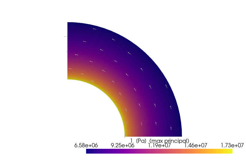
Principal stresses + principal directions on a thick cylinder

Where Nodal stress recovery + invariants — Lamé thick-walled cylinder answered how big the stress is, this example answers which way it points. The Cauchy stress tensor \(\sigma_{ij}\) at every node has three orthogonal principal directions along which there is no shear, with the corresponding principal stresses \(\sigma_{1} \ge \sigma_{2} \ge \sigma_{3}\) along those axes. Tracing those eigenvectors over a domain gives the stress-trajectory picture beloved by mechanical designers (Timoshenko & Goodier 1970 §1.7) — the visualisation that shows where the load actually flows.

For a thick cylinder under internal pressure, the answer is known exactly: the principal directions are radial and hoop, and \(\sigma_{1}\) is the hoop component everywhere. So the recovered eigenvectors give a clean accuracy check — they should point along the local \(\hat{\theta}\) to within mesh- discretisation error.

This example uses the public stress-recovery pipeline plus numpy.linalg.eigh() per node to extract the principal directions (stress_invariants returns the principal stresses only):

1. compute_nodal_stress(model, u) — node-averaged Voigt array.

2. stress_invariants(sigma) — \(\sigma_{1,2,3}\) and companion scalars per node.

3. np.linalg.eigh on the per-node 3x3 Cauchy tensor — yields sorted eigenvalues and eigenvectors so we can identify which principal axis aligns with which physical direction.

Verification

At every node of the Lamé annulus, the recovered \(\sigma_{1}\) direction must be tangent to the local hoop circle (perpendicular to the radial unit vector). We compute the angle between the recovered \(\sigma_{1}\) axis and the analytical hoop direction \(\hat{\theta}\) at every node and verify that it stays under a small tolerance — the trace error grows mildly with mesh size but never drifts off the hoop direction.

References

• Timoshenko, S. P. and Goodier, J. N. (1970) Theory of Elasticity, 3rd ed., McGraw-Hill, §1.7 — principal axes, §33 — Lamé thick cylinder.

• Cook, R. D., Malkus, D. S., Plesha, M. E., Witt, R. J. (2002) Concepts and Applications of Finite Element Analysis, 4th ed., Wiley, §3.6 — stress invariants and principal stresses.

• Sokolnikoff, I. S. (1956) Mathematical Theory of Elasticity, 2nd ed., McGraw-Hill, §22 — principal-direction trajectories.

from __future__ import annotations

import math

import numpy as np
import pyvista as pv

import femorph_solver
from femorph_solver import ELEMENTS
from femorph_solver.recover import compute_nodal_stress, stress_invariants

Build the Lamé quarter-annulus (HEX8 EAS, plane strain)

a = 0.10  # bore radius [m]
b = 0.20  # outer radius [m]
t_axial = 0.02  # plane-strain slab thickness [m]
p_i = 1.0e7  # internal pressure [Pa]
E = 2.0e11
NU = 0.30
N_THETA, N_RAD = 24, 16

theta = np.linspace(0.0, 0.5 * math.pi, N_THETA + 1)
r = np.linspace(a, b, N_RAD + 1)

pts_list: list[list[float]] = []
for kz in (0.0, t_axial):
    for ti in theta:
        for rj in r:
            pts_list.append([rj * math.cos(ti), rj * math.sin(ti), kz])
pts_arr = np.array(pts_list, dtype=np.float64)

nx_plane = (N_THETA + 1) * (N_RAD + 1)
n_cells = N_THETA * N_RAD
cells = np.empty((n_cells, 9), dtype=np.int64)
cells[:, 0] = 8
c = 0
for i in range(N_THETA):
    for j in range(N_RAD):
        n00b = i * (N_RAD + 1) + j
        n10b = i * (N_RAD + 1) + (j + 1)
        n11b = (i + 1) * (N_RAD + 1) + (j + 1)
        n01b = (i + 1) * (N_RAD + 1) + j
        cells[c, 1:] = (
            n00b,
            n10b,
            n11b,
            n01b,
            n00b + nx_plane,
            n10b + nx_plane,
            n11b + nx_plane,
            n01b + nx_plane,
        )
        c += 1
grid = pv.UnstructuredGrid(cells.ravel(), np.full(n_cells, 12, dtype=np.uint8), pts_arr)

m = femorph_solver.Model.from_grid(grid)
m.assign(
    ELEMENTS.HEX8(integration="enhanced_strain"),
    material={"EX": E, "PRXY": NU, "DENS": 7850.0},
)

for k, p in enumerate(pts_arr):
    if p[0] < 1e-9:
        m.fix(nodes=[int(k + 1)], dof="UX")
    if p[1] < 1e-9:
        m.fix(nodes=[int(k + 1)], dof="UY")
    m.fix(nodes=[int(k + 1)], dof="UZ")

# Internal pressure — lump as nodal forces on the bore face.
fx_acc: dict[int, float] = {}
fy_acc: dict[int, float] = {}
for kz in (0, 1):
    inner = [kz * nx_plane + i * (N_RAD + 1) + 0 for i in range(N_THETA + 1)]
    for seg in range(N_THETA):
        ai, bi = inner[seg], inner[seg + 1]
        ds = float(np.linalg.norm(pts_arr[bi] - pts_arr[ai]))
        mid = 0.5 * (pts_arr[ai] + pts_arr[bi])
        rxy = np.array([mid[0], mid[1]])
        nrm = float(np.linalg.norm(rxy))
        outward = rxy / nrm if nrm > 1e-12 else np.zeros(2)
        f_seg = p_i * ds * (t_axial / 2.0)
        for n_idx in (ai, bi):
            fx_acc[n_idx] = fx_acc.get(n_idx, 0.0) + 0.5 * f_seg * outward[0]
            fy_acc[n_idx] = fy_acc.get(n_idx, 0.0) + 0.5 * f_seg * outward[1]
for n_idx, fx in fx_acc.items():
    fy = fy_acc[n_idx]
    m.apply_force(int(n_idx + 1), fx=fx, fy=fy)

print("Lamé thick cylinder — principal stress + principal direction recovery")
print(f"  a = {a} m, b = {b} m, p_i = {p_i / 1e6:.1f} MPa, mesh ({N_THETA}, {N_RAD})")

Lamé thick cylinder — principal stress + principal direction recovery
  a = 0.1 m, b = 0.2 m, p_i = 10.0 MPa, mesh (24, 16)

Solve and recover the stress field

res = m.solve_static()
u = np.asarray(res.displacement, dtype=np.float64).ravel()
sigma = compute_nodal_stress(m, u)
inv = stress_invariants(sigma)

Recover the principal directions per node

stress_invariants returns the eigenvalues only; for principal directions we re-build the (n_points, 3, 3) Cauchy tensors and call np.linalg.eigh to get sorted eigenvalues and eigenvectors. eigh returns ascending eigenvalues, so column 2 is \(\sigma_{1}\).

n_pts = sigma.shape[0]
T = np.empty((n_pts, 3, 3), dtype=np.float64)
T[:, 0, 0] = sigma[:, 0]
T[:, 1, 1] = sigma[:, 1]
T[:, 2, 2] = sigma[:, 2]
T[:, 0, 1] = T[:, 1, 0] = sigma[:, 3]
T[:, 1, 2] = T[:, 2, 1] = sigma[:, 4]
T[:, 0, 2] = T[:, 2, 0] = sigma[:, 5]
eigvals, eigvecs = np.linalg.eigh(T)
# eigvecs[:, :, k] is the k-th eigenvector (ascending); k=2 → σ1.
v1 = eigvecs[:, :, 2]
v3 = eigvecs[:, :, 0]

Verify: σ1 axis aligns with the analytical hoop direction

At a point \((r\cos\theta, r\sin\theta, z)\) on the annulus, the hoop unit vector is \(\hat{\theta} = (-\sin\theta, \cos\theta, 0)\). The recovered \(\sigma_{1}\) eigenvector should be parallel (or anti-parallel) to it — alignment is the absolute dot product.

r_xy = np.linalg.norm(pts_arr[:, :2], axis=1)
theta_node = np.arctan2(pts_arr[:, 1], pts_arr[:, 0])
hoop_hat = np.column_stack([-np.sin(theta_node), np.cos(theta_node), np.zeros_like(theta_node)])
align = np.abs((v1 * hoop_hat).sum(axis=1))
# Skip the on-axis ridge (r ≈ 0) where the hoop direction is undefined.
mask = r_xy > 1e-6
mean_align = float(align[mask].mean())
worst_align = float(align[mask].min())
print(f"\n  σ1 / hoop alignment   mean |v1·θ̂| = {mean_align:.6f}   min = {worst_align:.6f}")
print(f"  worst-case angle off hoop:  {np.rad2deg(np.arccos(worst_align)):.3f}°")

assert mean_align > 0.999, f"σ1 axis drifted from hoop direction (mean alignment {mean_align:.6f})"
assert worst_align > 0.95, f"worst-case σ1 / hoop alignment {worst_align:.6f}"

σ1 / hoop alignment   mean |v1·θ̂| = 0.999989   min = 0.999866
worst-case angle off hoop:  0.938°

Tabulate principal stresses at the bore + outer radii

Closed form for the Lamé cylinder at any radius \(r\):

\[\sigma_\theta(r) = p_i \cdot \frac{a^2\,(b^2 + r^2)}{r^2\,(b^2 - a^2)}, \qquad \sigma_r(r) = -\,p_i \cdot \frac{a^2\,(b^2 - r^2)}{r^2\,(b^2 - a^2)}.\]

So \(\sigma_1 \approx \sigma_\theta\) (positive) and \(\sigma_3 \approx \sigma_r\) (negative) — at \(\theta = 0\) / \(\theta = \pi/2\) the radial and hoop directions trade with the global \(x / y\) axes.

print()
print(
    f"  {'r [m]':>7}  {'σ1 FE [MPa]':>13}  {'σ_θ pub [MPa]':>14}  "
    f"{'σ3 FE [MPa]':>13}  {'σ_r pub [MPa]':>14}"
)
print("  " + "-" * 64)
target_radii = (a, 0.5 * (a + b), b)
for r_target in target_radii:
    # First node closest to (r_target, 0, 0).
    diff = np.linalg.norm(pts_arr[:, :2] - np.array([r_target, 0.0]), axis=1)
    i_star = int(np.argmin(diff))
    sigma_theta_pub = p_i * a**2 * (b**2 + r_target**2) / (r_target**2 * (b**2 - a**2))
    sigma_r_pub = -p_i * a**2 * (b**2 - r_target**2) / (r_target**2 * (b**2 - a**2))
    print(
        f"  {r_target:>7.4f}  "
        f"{inv['s1'][i_star] / 1e6:>11.3f}  {sigma_theta_pub / 1e6:>13.3f}  "
        f"{inv['s3'][i_star] / 1e6:>11.3f}  {sigma_r_pub / 1e6:>13.3f}"
    )

  r [m]    σ1 FE [MPa]   σ_θ pub [MPa]    σ3 FE [MPa]   σ_r pub [MPa]
----------------------------------------------------------------
 0.1000       17.255         16.667       -8.624        -10.000
 0.1500        9.251          9.259       -2.611         -2.593
 0.2000        6.585          6.667       -0.189         -0.000

Render the σ1 field and principal-direction trajectories

grid_render = grid.copy()
grid_render.point_data["σ1 [Pa]"] = inv["s1"]
grid_render.point_data["σ3 [Pa]"] = inv["s3"]
grid_render.point_data["σ_VM [Pa]"] = inv["von_mises"]
grid_render.point_data["v1"] = v1
grid_render.point_data["v3"] = v3

# Sample every Mth node to keep the arrow plot readable.
sample_stride = max(1, n_pts // 64)
sample_idx = np.arange(0, n_pts, sample_stride)
arrow_pts = pts_arr[sample_idx]
arrow_v1 = v1[sample_idx]
# Scale arrows uniformly to ~6 % of the bounding box.
arrow_len = 0.06 * (b - a)

arrow_grid = pv.PolyData(arrow_pts)
arrow_grid["v1"] = arrow_v1
arrow_grid.set_active_vectors("v1")
arrows = arrow_grid.glyph(orient="v1", scale=False, factor=arrow_len)

plotter = pv.Plotter(off_screen=True, window_size=(820, 540))
plotter.add_mesh(
    grid_render,
    scalars="σ1 [Pa]",
    cmap="plasma",
    show_edges=False,
    scalar_bar_args={"title": "σ1  [Pa]  (max principal)"},
)
plotter.add_mesh(arrows, color="white", line_width=2)
plotter.view_xy()
plotter.camera.zoom(1.05)
plotter.show()

Take-aways

print()
print("Take-aways:")
print(
    "  • stress_invariants(sigma) returns the principal *stresses* (s1 ≥ s2 ≥ s3) "
    "along with von-Mises / hydrostatic / max-shear scalars.  Use it for any "
    "design check that needs σ1 (max tension) or σ3 (max compression)."
)
print(
    "  • Principal *directions* require the full eigendecomposition: build the "
    "per-node 3x3 Cauchy tensor and call np.linalg.eigh — eigvecs[:,:,2] is "
    "the σ1 axis."
)
print(
    "  • Plotting the σ1 eigenvector field on top of a stress contour gives the "
    "stress-trajectory picture: where the load actually flows.  At bore-edge "
    "in a Lamé cylinder the trajectories are perfect circles."
)
print(
    "  • Always sanity-check principal directions against an analytical reference "
    "where one exists (radial / hoop for cylinders, bending fibres for beams) — "
    "drift off the expected axis is an early warning of mesh or BC error."
)

Take-aways:
  • stress_invariants(sigma) returns the principal *stresses* (s1 ≥ s2 ≥ s3) along with von-Mises / hydrostatic / max-shear scalars.  Use it for any design check that needs σ1 (max tension) or σ3 (max compression).
  • Principal *directions* require the full eigendecomposition: build the per-node 3x3 Cauchy tensor and call np.linalg.eigh — eigvecs[:,:,2] is the σ1 axis.
  • Plotting the σ1 eigenvector field on top of a stress contour gives the stress-trajectory picture: where the load actually flows.  At bore-edge in a Lamé cylinder the trajectories are perfect circles.
  • Always sanity-check principal directions against an analytical reference where one exists (radial / hoop for cylinders, bending fibres for beams) — drift off the expected axis is an early warning of mesh or BC error.