Nodal stress recovery + invariants — Lamé thick-walled cylinder

Stress is the most-asked-for derived quantity in linear FEA, and the recovery from a displacement solution is where most of the “why is my stress field wrong” questions actually live. This example walks through the recovery pipeline on a problem with a clean closed-form reference — the Lamé thick cylinder under internal pressure (Timoshenko & Goodier 1970 §33) — so every intermediate quantity has an analytical value to compare against.

Two public post-processing helpers carry the work:

• femorph_solver.recover.compute_nodal_stress() — for each node, take the unweighted arithmetic mean of the per-element stress contributions evaluated at that node. Returns a (n_points, 6) Voigt array \((\sigma_{xx}, \sigma_{yy}, \sigma_{zz}, \sigma_{xy}, \sigma_{yz}, \sigma_{zx})\). The same call Result.stress drives.

• femorph_solver.recover.stress_invariants() — derive von Mises, hydrostatic, deviatoric, and principal stresses from a Voigt-stress array. Vectorised over the leading axis so stress_invariants(sigma_avg) returns a per-node table.

The closed-form Lamé hoop stress at the bore is

\[\sigma_{\theta}(a) \;=\; p_{i}\,\frac{a^{2} + b^{2}}{b^{2} - a^{2}},\]

(see Lamé thick-walled cylinder under internal pressure for the full derivation, and Mesh-refinement convergence — Lamé thick cylinder for the convergence plot).

This example reports the bore-edge \(\sigma_{\theta}\) for a three-point mesh-refinement ladder, so the role of mesh density on recovered stress is visible at a glance.

Implementation

Quarter-annulus HEX8 EAS plane-strain mesh — same setup as the verification benchmark. After each static solve we call:

• compute_nodal_stress() for the averaged Voigt-stress field.

• stress_invariants() to obtain the von-Mises / principal views of the same field.

References

• Timoshenko, S. P. and Goodier, J. N. (1970) Theory of Elasticity, 3rd ed., McGraw-Hill, §33.

• Cook, R. D., Malkus, D. S., Plesha, M. E., Witt, R. J. (2002) Concepts and Applications of Finite Element Analysis, 4th ed., Wiley, §6.12 — superconvergent stress recovery.

• Zienkiewicz, O. C. and Zhu, J. Z. (1992) “The superconvergent patch recovery and a-posteriori error estimates,” International Journal for Numerical Methods in Engineering 33 (7), 1331–1364 — the canonical “do better than averaging” paper.

from __future__ import annotations

import math

import numpy as np
import pyvista as pv

import femorph_solver
from femorph_solver import ELEMENTS
from femorph_solver.recover import compute_nodal_stress, stress_invariants

Problem data + closed-form reference

a = 0.10  # bore radius [m]
b = 0.20  # outer radius [m]
t_axial = 0.02  # plane-strain slab thickness [m]
p_i = 1.0e7  # internal pressure [Pa]
E = 2.0e11
NU = 0.30
RHO = 7850.0

sigma_theta_a_pub = p_i * (a**2 + b**2) / (b**2 - a**2)
sigma_r_a_pub = -p_i

print("Lamé thick cylinder — bore stress recovery via compute_nodal_stress")
print(f"  reference σ_θ(a) = {sigma_theta_a_pub / 1e6:7.3f} MPa  (Timoshenko & Goodier §33)")
print(f"  reference σ_r(a) = {sigma_r_a_pub / 1e6:7.3f} MPa  (= -p_i, exact)")


def build_solve_recover(
    n_theta: int, n_rad: int
) -> tuple[
    pv.UnstructuredGrid,
    np.ndarray,
    np.ndarray,
    np.ndarray,
]:
    """Build mesh, solve, and recover (σ_avg, σ_invariants, |u|)."""
    theta = np.linspace(0.0, 0.5 * math.pi, n_theta + 1)
    r = np.linspace(a, b, n_rad + 1)

    pts_list: list[list[float]] = []
    for kz in (0.0, t_axial):
        for ti in theta:
            for rj in r:
                pts_list.append([rj * math.cos(ti), rj * math.sin(ti), kz])
    pts_arr = np.array(pts_list, dtype=np.float64)

    nx_plane = (n_theta + 1) * (n_rad + 1)
    n_cells = n_theta * n_rad
    cells = np.empty((n_cells, 9), dtype=np.int64)
    cells[:, 0] = 8
    c = 0
    for i in range(n_theta):
        for j in range(n_rad):
            n00b = i * (n_rad + 1) + j
            n10b = i * (n_rad + 1) + (j + 1)
            n11b = (i + 1) * (n_rad + 1) + (j + 1)
            n01b = (i + 1) * (n_rad + 1) + j
            cells[c, 1:] = (
                n00b,
                n10b,
                n11b,
                n01b,
                n00b + nx_plane,
                n10b + nx_plane,
                n11b + nx_plane,
                n01b + nx_plane,
            )
            c += 1
    grid = pv.UnstructuredGrid(
        cells.ravel(),
        np.full(n_cells, 12, dtype=np.uint8),
        pts_arr,
    )

    m = femorph_solver.Model.from_grid(grid)
    m.assign(
        ELEMENTS.HEX8(integration="enhanced_strain"),
        material={"EX": E, "PRXY": NU, "DENS": RHO},
    )

    # Plane-strain BCs + symmetry pins.
    for k, p in enumerate(pts_arr):
        if p[0] < 1e-9:
            m.fix(nodes=[int(k + 1)], dof="UX")
        if p[1] < 1e-9:
            m.fix(nodes=[int(k + 1)], dof="UY")
        m.fix(nodes=[int(k + 1)], dof="UZ")

    # Internal-pressure load on the bore face.
    fx_acc: dict[int, float] = {}
    fy_acc: dict[int, float] = {}
    for kz in (0, 1):
        inner = [kz * nx_plane + i * (n_rad + 1) + 0 for i in range(n_theta + 1)]
        for seg in range(n_theta):
            ai, bi = inner[seg], inner[seg + 1]
            ds = float(np.linalg.norm(pts_arr[bi] - pts_arr[ai]))
            mid = 0.5 * (pts_arr[ai] + pts_arr[bi])
            rxy = np.array([mid[0], mid[1]])
            nrm = float(np.linalg.norm(rxy))
            outward = rxy / nrm if nrm > 1e-12 else np.zeros(2)
            f_seg = p_i * ds * (t_axial / 2.0)
            for n_idx in (ai, bi):
                fx_acc[n_idx] = fx_acc.get(n_idx, 0.0) + 0.5 * f_seg * outward[0]
                fy_acc[n_idx] = fy_acc.get(n_idx, 0.0) + 0.5 * f_seg * outward[1]
    for n_idx, fx in fx_acc.items():
        fy = fy_acc[n_idx]
        m.apply_force(int(n_idx + 1), fx=fx, fy=fy)

    res = m.solve_static()
    u = np.asarray(res.displacement, dtype=np.float64).ravel()
    sigma = compute_nodal_stress(m, u)
    invariants = stress_invariants(sigma)
    u_mag = np.linalg.norm(u.reshape(-1, 3), axis=1)
    grid_with_data = grid.copy()
    grid_with_data.point_data["sigma_xx"] = sigma[:, 0]
    grid_with_data.point_data["sigma_yy"] = sigma[:, 1]
    grid_with_data.point_data["sigma_vm"] = invariants["von_mises"]
    grid_with_data.point_data["s1"] = invariants["s1"]
    grid_with_data.point_data["|u|"] = u_mag
    grid_with_data.point_data["displacement"] = u.reshape(-1, 3)
    return grid_with_data, sigma, invariants, pts_arr

Lamé thick cylinder — bore stress recovery via compute_nodal_stress
  reference σ_θ(a) =  16.667 MPa  (Timoshenko & Goodier §33)
  reference σ_r(a) = -10.000 MPa  (= -p_i, exact)

Mesh-refinement ladder

The recovered \(\sigma_{\theta}\) at the bore converges from below as the mesh refines. At the equator (θ=0) the radial direction is \(+x\) and the hoop is \(+y\), so we read \(\sigma_{\theta}\) off as \(\sigma_{yy}\).

print()
print(
    f"  {'(N_θ, N_r)':>11}  {'σ_θ FE [MPa]':>14}  {'err vs pub':>11}  "
    f"{'σ_r FE [MPa]':>14}  {'σ_VM at bore [MPa]':>20}"
)
print(f"  {'-' * 11:>11}  {'-' * 14:>14}  {'-' * 11:>11}  {'-' * 14:>14}  {'-' * 20:>20}")

ladder = ((12, 8), (24, 16), (36, 24))
last_grid = None
last_pts = None
for n_th, n_r in ladder:
    g_, sigma_, inv_, pts_ = build_solve_recover(n_th, n_r)
    i_bore = int(np.argmin(np.linalg.norm(pts_ - np.array([a, 0.0, 0.0]), axis=1)))
    s_yy = float(sigma_[i_bore, 1])
    s_xx = float(sigma_[i_bore, 0])
    s_vm = float(inv_["von_mises"][i_bore])
    err = (s_yy - sigma_theta_a_pub) / sigma_theta_a_pub * 100.0
    print(
        f"  ({n_th:>3}, {n_r:>3})  {s_yy / 1e6:>12.3f}  "
        f"{err:>+10.3f}%  {s_xx / 1e6:>12.3f}  {s_vm / 1e6:>18.3f}"
    )
    last_grid = g_
    last_pts = pts_

 (N_θ, N_r)    σ_θ FE [MPa]   err vs pub    σ_r FE [MPa]    σ_VM at bore [MPa]
-----------  --------------  -----------  --------------  --------------------
( 12,   8)        17.750      +6.499%        -7.370              21.900
( 24,  16)        17.248      +3.491%        -8.617              22.478
( 36,  24)        17.064      +2.383%        -9.062              22.687

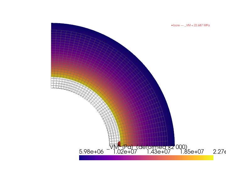
Render the σ_VM (von Mises) field on the finest mesh

stress_invariants returns the full set of derived scalars in one pass; here we render the von-Mises field which is the combined-stress measure design codes most often gate against.

assert last_grid is not None
assert last_pts is not None
i_bore = int(np.argmin(np.linalg.norm(last_pts - np.array([a, 0.0, 0.0]), axis=1)))
warped = last_grid.warp_by_vector("displacement", factor=2.0e3)

plotter = pv.Plotter(off_screen=True, window_size=(720, 540))
plotter.add_mesh(last_grid, style="wireframe", color="grey", opacity=0.35, line_width=1)
plotter.add_mesh(
    warped,
    scalars="sigma_vm",
    cmap="plasma",
    show_edges=False,
    scalar_bar_args={"title": "σ_VM  [Pa]  (deformed ×2 000)"},
)
disp = np.asarray(last_grid.point_data["displacement"])
plotter.add_points(
    last_pts[i_bore : i_bore + 1] + 2.0e3 * disp[i_bore],
    render_points_as_spheres=True,
    point_size=18,
    color="#d62728",
    label=f"bore — σ_VM = {last_grid.point_data['sigma_vm'][i_bore] / 1e6:.3f} MPa",
)
plotter.add_legend()
plotter.view_xy()
plotter.camera.zoom(1.05)
plotter.show()

Take-aways

print()
print("Take-aways:")
print(
    "  • compute_nodal_stress(m, u) returns a (n_points, 6) Voigt array of "
    "node-averaged stress.  Same call Result.stress drives."
)
print(
    "  • stress_invariants(sigma) is vectorised — pass a per-node array, "
    "get a dict of per-node von-Mises / principal / hydrostatic / deviatoric scalars."
)
print(
    "  • Recovered σ_θ converges to the closed form from below — coarse meshes "
    "under-predict at the bore because the steep radial gradient is poorly "
    "represented by trilinear shape functions on the inner ring of elements."
)
print(
    "  • Stress is always less accurate than displacement on the same mesh "
    "(d = O(h²), σ = O(h) for HEX8); see "
    ":ref:`sphx_glr_gallery_verification_example_verify_convergence_lame.py` "
    "for the full convergence curve."
)

Take-aways:
  • compute_nodal_stress(m, u) returns a (n_points, 6) Voigt array of node-averaged stress.  Same call Result.stress drives.
  • stress_invariants(sigma) is vectorised — pass a per-node array, get a dict of per-node von-Mises / principal / hydrostatic / deviatoric scalars.
  • Recovered σ_θ converges to the closed form from below — coarse meshes under-predict at the bore because the steep radial gradient is poorly represented by trilinear shape functions on the inner ring of elements.
  • Stress is always less accurate than displacement on the same mesh (d = O(h²), σ = O(h) for HEX8); see :ref:`sphx_glr_gallery_verification_example_verify_convergence_lame.py` for the full convergence curve.