Note
Go to the end to download the full example code.
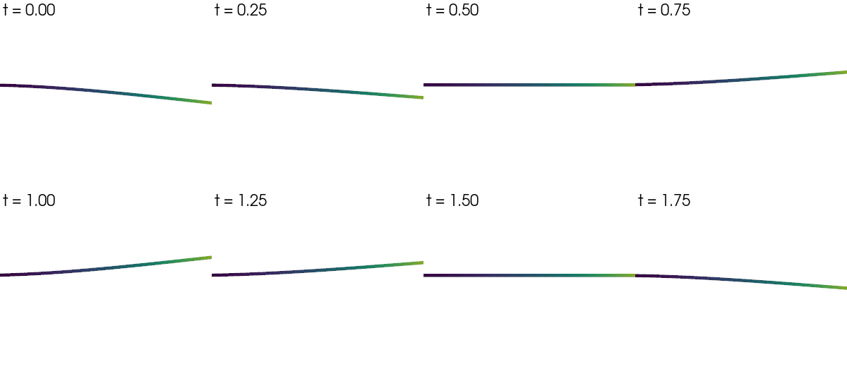
Mode-shape animation — cantilever bending modes#
A mode shape \(\phi_{i}\) is the spatial pattern of a structure’s \(i\)-th free-vibration response. When the structure is excited at the corresponding natural frequency \(f_{i}\), every point moves in phase with amplitude proportional to \(\phi_{i}\) and time profile
So an “animation” of mode \(i\) is just a parametric sweep over phase \(\omega t \in [0, 2\pi]\), with the displacement field scaled by \(\cos(\omega t)\) at each frame. The static plot Plotting mode shapes shows one snapshot per mode; this example shows the time evolution of a single mode across one full period — the key visual that makes mode shapes click for new users.
The standard recipe:
modal_result_to_grid(model, result)scatters every mode onto the mesh as amode_{k}_disppoint-data vector.For each animation frame,
grid.warp_by_vector("mode_k_disp",
factor=A·cos(ωt))
deforms the geometry by the phase-scaled shape.Render either as a filmstrip (sphinx-gallery friendly) or as a true GIF/MP4 with
pyvista.Plotter.open_gif()/pyvista.Plotter.write_frame().
Step 3 is the only one that branches: the gallery shows a filmstrip
because the doc build is offscreen, but the script writes a GIF too —
running this file locally produces mode_1_animation.gif next to
the source.
Implementation#
Slender HEX8 cantilever (clamped at \(x = 0\)). Solve six modes, pick mode 1 (first transverse bending), filmstrip eight evenly-spaced phases over one period. Mode-shape amplitude is normalised so the peak displacement reaches 8 % of the beam length — a visually readable scale that is also physically meaningless (mode shapes carry no absolute magnitude; the norm choice is arbitrary).
References#
Bathe, K.-J. (2014) Finite Element Procedures, 2nd ed., Prentice Hall, §10.2 — undamped free vibration.
Chopra, A. K. (2017) Dynamics of Structures, 5th ed., Pearson, §10.2 — free-vibration response of MDOF systems.
Cook, R. D., Malkus, D. S., Plesha, M. E., Witt, R. J. (2002) Concepts and Applications of Finite Element Analysis, 4th ed., Wiley, §11.3 — eigenproblems of structural dynamics.
from __future__ import annotations

from pathlib import Path

import numpy as np
import pyvista as pv

import femorph_solver
from femorph_solver import ELEMENTS
from femorph_solver.io import modal_result_to_grid
Build a slender cantilever beam (HEX8 EAS)#
E = 2.0e11
NU = 0.30
RHO = 7850.0
L = 4.0
WIDTH = 0.05
HEIGHT = 0.05

NX, NY, NZ = 60, 3, 3
xs = np.linspace(0.0, L, NX + 1)
ys = np.linspace(0.0, WIDTH, NY + 1)
zs = np.linspace(0.0, HEIGHT, NZ + 1)
grid = pv.StructuredGrid(*np.meshgrid(xs, ys, zs, indexing="ij")).cast_to_unstructured_grid()

m = femorph_solver.Model.from_grid(grid)
m.assign(
    ELEMENTS.HEX8(integration="enhanced_strain"),
    material={"EX": E, "PRXY": NU, "DENS": RHO},
)

pts = np.asarray(m.grid.points)
clamped = np.where(pts[:, 0] < 1e-9)[0]
m.fix(nodes=(clamped + 1).tolist(), dof="ALL")
Modal solve + scatter onto the grid#
N_MODES = 6
res = m.solve_modal(n_modes=N_MODES)
freqs = np.asarray(res.frequency, dtype=np.float64)
print("Cantilever beam — first six natural frequencies")
for i, f in enumerate(freqs):
    print(f"  mode {i + 1}:  f = {f:7.3f} Hz")

# ``modal_result_to_grid`` attaches one ``mode_{k}_disp`` vector and
# one ``mode_{k}_magnitude`` scalar per mode.  ``scale`` is uniform —
# we'll choose a per-mode amplitude later when we render.
grid_modes = modal_result_to_grid(m, res, scale=1.0)
Cantilever beam — first six natural frequencies
  mode 1:  f =   2.554 Hz
  mode 2:  f =   2.554 Hz
  mode 3:  f =  16.005 Hz
  mode 4:  f =  16.005 Hz
  mode 5:  f =  44.825 Hz
  mode 6:  f =  44.825 Hz
Pick the visualisation amplitude#
Mode shapes are mass-normalised, so the magnitudes look tiny in absolute units. Pick a render amplitude such that the peak displacement equals 8 % of the beam length — independent of the eigenvector norm, this gives a consistent visual.
mode_index = 1  # animate mode 1 (first transverse bending)
disp = np.asarray(grid_modes.point_data[f"mode_{mode_index}_disp"])
peak = float(np.linalg.norm(disp, axis=1).max())
target_peak = 0.08 * L  # 8 % of beam length
amp = target_peak / peak if peak > 0 else 1.0
print(
    f"\n  Animating mode {mode_index} at f = {freqs[mode_index - 1]:.3f} Hz, "
    f"amplitude scaled so peak displacement = {target_peak:.3f} m "
    f"({100 * target_peak / L:.1f}% of L)"
)
Animating mode 1 at f = 2.554 Hz, amplitude scaled so peak displacement = 0.320 m (8.0% of L)
Filmstrip: eight phase snapshots over one period#
Sphinx-gallery captures static images, so the rendered output is a
2 x 4 filmstrip of warps at ωt = 0, π/4, π/2, …, 7π/4. Running
this script locally also writes a real GIF — see the next cell.
n_frames = 8
phases = np.linspace(0.0, 2.0 * np.pi, n_frames, endpoint=False)

plotter = pv.Plotter(shape=(2, 4), off_screen=True, window_size=(1200, 540), border=False)
for k, phase in enumerate(phases):
    row, col = divmod(k, 4)
    plotter.subplot(row, col)
    factor = amp * float(np.cos(phase))
    warped = grid_modes.warp_by_vector(f"mode_{mode_index}_disp", factor=factor)
    plotter.add_mesh(
        warped,
        scalars=f"mode_{mode_index}_magnitude",
        cmap="viridis",
        clim=(0.0, peak),
        show_edges=False,
        show_scalar_bar=False,
    )
    plotter.add_text(f"ωt = {phase / np.pi:.2f}π", position="upper_left", font_size=10)
    plotter.view_xy()
    plotter.camera.zoom(1.4)
plotter.link_views()
plotter.show()
Write a real GIF for users running this script directly#
The block below produces a 24-frame GIF that loops over one full period —
this is the artefact you actually want to embed in a report or a slide.
Sphinx-gallery captures only the static filmstrip above, so the GIF lands
in tempfile.gettempdir() rather than the source tree (the printed
path tells you exactly where). GIF writing uses pyvista’s
open_gif() / write_frame()
pair and requires imageio (already pulled in by pyvista).
import importlib.util  # noqa: E402
import tempfile  # noqa: E402

if importlib.util.find_spec("imageio") is None:
    print(
        "\n  imageio not installed — skipping GIF write.  "
        "Install with `pip install imageio` to enable Plotter.open_gif."
    )
else:
    out_path = Path(tempfile.gettempdir()) / f"mode_{mode_index}_animation.gif"
    n_gif_frames = 24
    gif_phases = np.linspace(0.0, 2.0 * np.pi, n_gif_frames, endpoint=False)

    p2 = pv.Plotter(off_screen=True, window_size=(720, 480))
    p2.view_xy()
    p2.camera.zoom(1.3)
    p2.open_gif(str(out_path))
    for phase in gif_phases:
        p2.clear_actors()
        factor = amp * float(np.cos(phase))
        warped = grid_modes.warp_by_vector(f"mode_{mode_index}_disp", factor=factor)
        p2.add_mesh(
            warped,
            scalars=f"mode_{mode_index}_magnitude",
            cmap="viridis",
            clim=(0.0, peak),
            show_edges=False,
            show_scalar_bar=False,
        )
        p2.add_text(
            f"mode {mode_index}  —  f = {freqs[mode_index - 1]:.2f} Hz",
            position="upper_left",
            font_size=11,
        )
        p2.write_frame()
    p2.close()
    print(f"\n  GIF written to {out_path}")
imageio not installed — skipping GIF write. Install with `pip install imageio` to enable Plotter.open_gif.
Take-aways#
print()
print("Take-aways:")
print(
    "  • A mode shape is a spatial pattern; its time evolution at the natural "
    "frequency is u(x,t) = A·φ(x)·cos(2π f t).  Animation = phase sweep over "
    "ωt ∈ [0, 2π]."
)
print(
    "  • modal_result_to_grid(m, res) attaches per-mode vector arrays "
    "(mode_k_disp); pyvista's warp_by_vector(factor=A·cos(ωt)) deforms the "
    "mesh by the phase-scaled shape."
)
print(
    "  • Mode-shape magnitudes are arbitrary (mass-normalised eigenvectors).  "
    "Pick the render amplitude to be a fraction of the structure's bounding "
    "box — never raw eigenvector units."
)
print(
    "  • For a true animation, use Plotter.open_gif(path) + write_frame() in "
    "an off-screen plotter; the same loop that fills the filmstrip produces "
    "the GIF frames."
)
Take-aways:
  • A mode shape is a spatial pattern; its time evolution at the natural frequency is u(x,t) = A·φ(x)·cos(2π f t).  Animation = phase sweep over ωt ∈ [0, 2π].
  • modal_result_to_grid(m, res) attaches per-mode vector arrays (mode_k_disp); pyvista's warp_by_vector(factor=A·cos(ωt)) deforms the mesh by the phase-scaled shape.
  • Mode-shape magnitudes are arbitrary (mass-normalised eigenvectors).  Pick the render amplitude to be a fraction of the structure's bounding box — never raw eigenvector units.
  • For a true animation, use Plotter.open_gif(path) + write_frame() in an off-screen plotter; the same loop that fills the filmstrip produces the GIF frames.
Total running time of the script: (0 minutes 0.754 seconds)