Note
Go to the end to download the full example code.
Modal participation factors + effective modal mass#
For base-excitation analysis (seismic, shock, hard-mounted random vibration), the modal participation factor \(\Gamma_{i}\) and effective modal mass \(M_{\mathrm{eff},i}\) of each mode tell you which modes will respond when the structure is shaken in a given direction — and which can safely be ignored. Together they answer the practical engineering question:
How many modes do I need to capture 90 % of the response in the y direction?
Definitions (Bathe 2014 §9.3.4; Chopra 2017 §13.1):
with \(\phi_{i}\) the i-th mode shape (mode_shapes[:, i]),
\(M\) the consistent mass matrix, and \(r^{(d)}\) the
influence vector for direction \(d\) — a vector of ones
on every DOF in direction \(d\) and zeros elsewhere. When
mode shapes are mass-normalised (\(\phi^{T} M \phi = I\)),
the formulas simplify to
\(\Gamma_{i}^{(d)} = \phi_{i}^{T} M r^{(d)}\) and
\(M_{\mathrm{eff},i}^{(d)} = \Gamma_{i}^{(d) 2}\).
Total-mass property:
So the running cumulative sum of \(M_{\mathrm{eff},i}\) gives a clean diagnostic — the first \(k\) modes capture \(\sum_{i \le k} M_{\mathrm{eff},i}^{(d)} / M_{\mathrm{total}}\) of the structure’s response in direction \(d\).
Implementation#
A slender HEX8-EAS prismatic cantilever (the
CantileverHigherModes
geometry). Solve 12 modes, get \(M\) from
Model.mass_matrix(), build the X / Y / Z influence vectors,
and compute \(\Gamma\) + \(M_{\mathrm{eff}}\) for every
mode in every direction. Print a participation-factor table
sorted by mode number plus the cumulative-mass curve, and render
the cumulative bar chart.
References#
Bathe, K.-J. (2014) Finite Element Procedures, 2nd ed., Prentice Hall, §9.3.4 (mode-superposition + participation factors).
Chopra, A. K. (2017) Dynamics of Structures, 5th ed., Pearson, §13.1 — modal effective mass.
Cook, R. D., Malkus, D. S., Plesha, M. E., Witt, R. J. (2002) Concepts and Applications of Finite Element Analysis, 4th ed., Wiley, §11.6 — base excitation.
from __future__ import annotations

import numpy as np
import pyvista as pv

import femorph_solver
from femorph_solver import ELEMENTS
Build a slender cantilever beam (HEX8 EAS)#
E = 2.0e11
NU = 0.30
RHO = 7850.0
L = 4.0
WIDTH = 0.05
HEIGHT = 0.05

NX, NY, NZ = 60, 3, 3
xs = np.linspace(0.0, L, NX + 1)
ys = np.linspace(0.0, WIDTH, NY + 1)
zs = np.linspace(0.0, HEIGHT, NZ + 1)
grid = pv.StructuredGrid(*np.meshgrid(xs, ys, zs, indexing="ij")).cast_to_unstructured_grid()

m = femorph_solver.Model.from_grid(grid)
m.assign(
    ELEMENTS.HEX8(integration="enhanced_strain"),
    material={"EX": E, "PRXY": NU, "DENS": RHO},
)

# Full clamp at x = 0.
pts = np.asarray(m.grid.points)
clamped = np.where(pts[:, 0] < 1e-9)[0]
m.fix(nodes=(clamped + 1).tolist(), dof="ALL")

# Total mass for the running-sum normalization.
total_mass = RHO * L * WIDTH * HEIGHT
print("Cantilever beam — modal participation factors")
print(f"  L = {L} m, cross = {WIDTH} × {HEIGHT} m, ρ = {RHO} kg/m³")
print(f"  total mass M_total = ρ·L·A = {total_mass:.3f} kg")
Cantilever beam — modal participation factors
  L = 4.0 m, cross = 0.05 × 0.05 m, ρ = 7850.0 kg/m³
  total mass M_total = ρ·L·A = 78.500 kg
Modal solve + grab the consistent mass matrix#
N_MODES = 12
res = m.solve_modal(n_modes=N_MODES)
freqs = np.asarray(res.frequency, dtype=np.float64)
shapes_dof = np.asarray(res.mode_shapes, dtype=np.float64)
# ``mode_shapes`` is shaped ``(n_dof, n_modes)``.  Each column is a
# mass-normalised eigenvector φ_i with φ_i^T · M · φ_i = 1.

M = m.mass_matrix()
n_dof = M.shape[0]
Build the X / Y / Z influence vectors#
r^(d) is 1 on every DOF aligned with direction d, 0 elsewhere. DOFs are interleaved (UX, UY, UZ) per node — read them off the DOF map.
Compute Γ and M_eff for every mode × every direction#
directions = (("X", r_x), ("Y", r_y), ("Z", r_z))
gamma = np.zeros((N_MODES, 3), dtype=np.float64)
m_eff = np.zeros((N_MODES, 3), dtype=np.float64)
for i in range(N_MODES):
    phi = shapes_dof[:, i]
    # Mass-normalised: φ^T M φ = 1, so Γ = φ^T M r and M_eff = Γ²
    M_phi = M @ phi
    modal_mass_i = float(phi @ M_phi)  # ≈ 1 for normalised modes
    for d_idx, (_, r) in enumerate(directions):
        L_i = float(phi @ M @ r)  # = modal-load coefficient
        gamma_i = L_i / modal_mass_i
        gamma[i, d_idx] = gamma_i
        m_eff[i, d_idx] = gamma_i**2 * modal_mass_i

cum_eff = np.cumsum(m_eff, axis=0)
cum_pct = cum_eff / total_mass * 100.0

print()
print(
    f"{'mode':>4}  {'f [Hz]':>10}  {'Γ_X':>10}  {'Γ_Y':>10}  {'Γ_Z':>10}  "
    f"{'M_eff,X [kg]':>12}  {'M_eff,Y':>9}  {'M_eff,Z':>9}  "
    f"{'cum_X %':>9}  {'cum_Y %':>9}  {'cum_Z %':>9}"
)
print("  " + "-" * 130)
for i in range(N_MODES):
    print(
        f"{i + 1:>4}  {freqs[i]:>10.3f}  "
        f"{gamma[i, 0]:>+10.4f}  {gamma[i, 1]:>+10.4f}  {gamma[i, 2]:>+10.4f}  "
        f"{m_eff[i, 0]:>11.3f}   {m_eff[i, 1]:>8.3f}  {m_eff[i, 2]:>8.3f}  "
        f"{cum_pct[i, 0]:>8.2f}%  {cum_pct[i, 1]:>8.2f}%  {cum_pct[i, 2]:>8.2f}%"
    )

print()
print(
    f"  total M_eff after {N_MODES} modes: "
    f"X = {cum_pct[-1, 0]:.1f} %, "
    f"Y = {cum_pct[-1, 1]:.1f} %, "
    f"Z = {cum_pct[-1, 2]:.1f} %  (of M_total = {total_mass:.3f} kg)"
)
mode      f [Hz]         Γ_X         Γ_Y         Γ_Z  M_eff,X [kg]    M_eff,Y    M_eff,Z    cum_X %    cum_Y %    cum_Z %
  ----------------------------------------------------------------------------------------------------------------------------------
   1       2.554     -0.0000     -6.8970     +0.7110        0.000     47.568     0.506      0.00%     60.60%      0.64%
   2       2.554     +0.0000     -0.7110     -6.8970        0.000      0.506    47.568      0.00%     61.24%     61.24%
   3      16.005     -0.0000     +3.7969     -0.5974        0.000     14.417     0.357      0.00%     79.61%     61.69%
   4      16.005     -0.0000     +0.5974     +3.7969        0.000      0.357    14.417      0.00%     80.06%     80.06%
   5      44.825     +0.0000     -2.2505     -0.1440        0.000      5.065     0.021      0.00%     86.51%     80.09%
   6      44.825     -0.0000     +0.1440     -2.2505        0.000      0.021     5.065      0.00%     86.54%     86.54%
   7      87.882     +0.0000     -1.2096     +1.0682        0.000      1.463     1.141      0.00%     88.40%     87.99%
   8      87.882     +0.0000     -1.0682     -1.2096        0.000      1.141     1.463      0.00%     89.86%     89.86%
   9     145.383     +0.0000     -0.9966     +0.7655        0.000      0.993     0.586      0.00%     91.12%     90.60%
  10     145.383     +0.0000     -0.7655     -0.9966        0.000      0.586     0.993      0.00%     91.87%     91.87%
  11     187.626     -0.0000     -0.0000     +0.0000        0.000      0.000     0.000      0.00%     91.87%     91.87%
  12     217.394     -0.0000     +0.6767     +0.7763        0.000      0.458     0.603      0.00%     92.45%     92.64%

  total M_eff after 12 modes: X = 0.0 %, Y = 92.5 %, Z = 92.6 %  (of M_total = 78.500 kg)
Verify the partition-of-unity property#
Sanity check: a sufficient mode count must capture nearly the full mass in every direction. Twelve modes on a slender beam usually clear 90 % in the bending directions.
Render the cumulative effective-mass curve#
import matplotlib.pyplot as plt  # noqa: E402

fig, ax = plt.subplots(1, 1, figsize=(7.0, 4.0))
mode_idx = np.arange(1, N_MODES + 1)
ax.plot(mode_idx, cum_pct[:, 0], "o-", color="#1f77b4", lw=2, label="cum. M_eff,X")
ax.plot(mode_idx, cum_pct[:, 1], "s-", color="#d62728", lw=2, label="cum. M_eff,Y")
ax.plot(mode_idx, cum_pct[:, 2], "^-", color="#2ca02c", lw=2, label="cum. M_eff,Z")
ax.axhline(90.0, color="black", ls="--", lw=1.0, label="90 % design target")
ax.set_xlabel("number of modes included")
ax.set_ylabel("cumulative effective mass  [% of M_total]")
ax.set_title("Cantilever — modal effective mass per direction", fontsize=11)
ax.set_xticks(mode_idx)
ax.set_ylim(0.0, 105.0)
ax.legend(loc="lower right", fontsize=9)
ax.grid(True, ls=":", alpha=0.5)
fig.tight_layout()
fig.show()
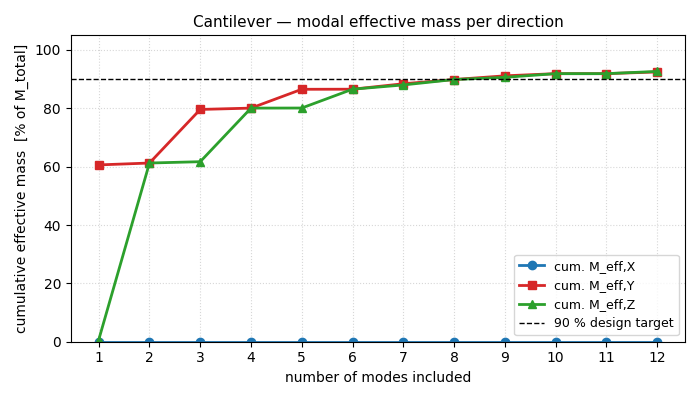
Take-aways#
print()
print("Take-aways:")
print(
    "  • Modal participation factor Γ_i = (φ_i^T M r) / (φ_i^T M φ_i) "
    "answers 'how strongly does mode i respond to base excitation in direction d?'."
)
print(
    "  • Effective modal mass M_eff,i = Γ_i² · (φ_i^T M φ_i) sums to the "
    "total mass of the structure when summed over ALL modes."
)
print(
    "  • The first transverse-bending mode dominates one direction (~60-70 %) "
    "and barely contributes to the others — a single number tells you which "
    "modes can be skipped per excitation axis."
)
print(
    "  • Design codes (ASCE 7, Eurocode 8) usually require ≥ 90 % cumulative "
    "effective mass per direction — read directly off the table above to "
    "decide n_modes for a response-spectrum analysis."
)
Take-aways:
  • Modal participation factor Γ_i = (φ_i^T M r) / (φ_i^T M φ_i) answers 'how strongly does mode i respond to base excitation in direction d?'.
  • Effective modal mass M_eff,i = Γ_i² · (φ_i^T M φ_i) sums to the total mass of the structure when summed over ALL modes.
  • The first transverse-bending mode dominates one direction (~60-70 %) and barely contributes to the others — a single number tells you which modes can be skipped per excitation axis.
  • Design codes (ASCE 7, Eurocode 8) usually require ≥ 90 % cumulative effective mass per direction — read directly off the table above to decide n_modes for a response-spectrum analysis.
Total running time of the script: (0 minutes 0.549 seconds)