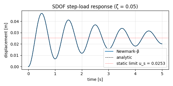
SDOF transient — step-load response

A single-DOF mass-spring-damper subjected to a step load shows off the Newmark-β transient integrator in solve_transient(). We integrate for long enough to watch the underdamped oscillation settle toward the new static equilibrium, then compare the result to the textbook second-order response.

from __future__ import annotations

import matplotlib.pyplot as plt
import numpy as np
import scipy.sparse as sp

from femorph_solver.solvers.transient import solve_transient

Set up a 1-DOF oscillator

m = 1.0  # kg
k = 4.0 * np.pi**2  # N / m — gives ωn = 2π rad/s (fn = 1 Hz)
zeta = 0.05
c = 2.0 * zeta * np.sqrt(k * m)

M = sp.csr_array(np.array([[m]], dtype=float))
K = sp.csr_array(np.array([[k]], dtype=float))
C = sp.csr_array(np.array([[c]], dtype=float))

Step load at t = 0

F_step = 1.0  # N
F = np.array([F_step])

Newmark-β with the default unconditionally-stable parameters

dt = 1e-3
n_steps = 5000
result = solve_transient(K, M, F, dt=dt, n_steps=n_steps, C=C)
u_fs = result.displacement[:, 0]

Analytical comparison

omega_n = np.sqrt(k / m)
omega_d = omega_n * np.sqrt(1 - zeta**2)
u_static = F_step / k
phi = np.arctan(zeta / np.sqrt(1 - zeta**2))
u_exact = u_static * (
    1
    - np.exp(-zeta * omega_n * result.time)
    / np.sqrt(1 - zeta**2)
    * np.cos(omega_d * result.time - phi)
)

Plot Newmark vs analytic

fig, ax = plt.subplots(figsize=(6, 3))
ax.plot(result.time, u_fs, label="Newmark-β", color="#1f77b4")
ax.plot(result.time, u_exact, "--", label="analytic", color="black", linewidth=0.8)
ax.axhline(
    u_static,
    color="red",
    linestyle=":",
    linewidth=0.8,
    label=f"static limit u_s = {u_static:.4f}",
)
ax.set_xlabel("time [s]")
ax.set_ylabel("displacement [m]")
ax.set_title("SDOF step-load response (ζ = 0.05)")
ax.legend(loc="lower right")
ax.grid(True, alpha=0.3)
fig.tight_layout()

err = np.max(np.abs(u_fs - u_exact)) / u_static
print(f"max relative error vs analytic: {err:.3e}")

max relative error vs analytic: 2.423e-05