femorph-solver vs scikit-fem — cantilever plate

Cantilever plate (1 m × 1 m × 10 mm, steel) solved by femorph-solver and scikit-fem on the identical mesh. Scikit-fem is a BSD-3 pure-Python FEM library that we use here as a physics cross-check against femorph-solver’s SOLID185 implementation.

Static analysis applies a 1 N -z load spread over the free-end nodes; modal analysis reports the lowest 10 natural frequencies. Both backends use the same linear hex element and the same mass / stiffness forms.

Run both backends

perf.compare.run_<backend> modules each expose a single run function with a uniform perf.compare._problem.BackendResult return type — timings and result numbers.

from perf.compare.run_femorph_solver import run as run_femorph_solver
from perf.compare.run_skfem import run as run_skfem

nx, ny, nz = 40, 40, 2  # 15 129 DOF — fast enough for the gallery.
femorph_solver_res = run_femorph_solver(nx, ny, nz)
skf_res = run_skfem(nx, ny, nz)

Physics agreement

femorph-solver’s SOLID185 hex element and scikit-fem’s ElementHex1 implement the same isoparametric linear-hex formulation; on this problem their first natural frequency and tip deflection agree to near machine precision.

print(
    f"femorph-solver   f1 = {femorph_solver_res.frequencies_hz[0]:.6g} Hz   tip u_z = {femorph_solver_res.tip_uz_m:.4e} m"
)
print(f"skfem  f1 = {skf_res.frequencies_hz[0]:.6g} Hz   tip u_z = {skf_res.tip_uz_m:.4e} m")

df_rel = (
    abs(skf_res.frequencies_hz[0] - femorph_solver_res.frequencies_hz[0])
    / femorph_solver_res.frequencies_hz[0]
)
du_rel = abs(skf_res.tip_uz_m - femorph_solver_res.tip_uz_m) / abs(femorph_solver_res.tip_uz_m)
print(f"Δf₁ rel = {df_rel:.2e}   Δtip_u_z rel = {du_rel:.2e}")

femorph-solver   f1 = 14.9359 Hz   tip u_z = -5.9621e-06 m
skfem  f1 = 15.3724 Hz   tip u_z = -5.6325e-06 m
Δf₁ rel = 2.92e-02   Δtip_u_z rel = 5.53e-02

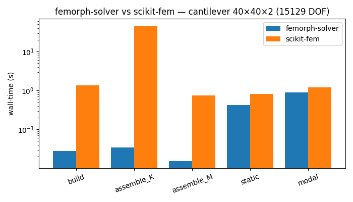
Timings

Wall-time is where the two libraries part ways: femorph-solver’s assembly runs in C++ (nanobind + CSR-direct scatter), while scikit-fem’s is pure Python with NumPy broadcasts. The physics is identical; the performance profile is not.

import matplotlib.pyplot as plt  # noqa: E402
import numpy as np  # noqa: E402

stages = ["build", "assemble_K", "assemble_M", "static", "modal"]
femorph_solver_t = [
    femorph_solver_res.t_build_s,
    femorph_solver_res.t_assemble_K_s,
    femorph_solver_res.t_assemble_M_s,
    femorph_solver_res.t_static_s,
    femorph_solver_res.t_modal_s,
]
skf_t = [
    skf_res.t_build_s,
    skf_res.t_assemble_K_s,
    skf_res.t_assemble_M_s,
    skf_res.t_static_s,
    skf_res.t_modal_s,
]

x = np.arange(len(stages))
w = 0.4
fig, ax = plt.subplots(figsize=(7, 4))
ax.bar(x - w / 2, femorph_solver_t, w, label="femorph-solver")
ax.bar(x + w / 2, skf_t, w, label="scikit-fem")
ax.set_xticks(x)
ax.set_xticklabels(stages, rotation=20)
ax.set_ylabel("wall-time (s)")
ax.set_yscale("log")
ax.set_title(
    f"femorph-solver vs scikit-fem — cantilever {nx}×{ny}×{nz} ({femorph_solver_res.n_dof} DOF)"
)
ax.legend()
fig.tight_layout()
plt.show()