femorph-solver vs scikit-fem — mesh-size scaling

Runs both backends across a range of in-plane mesh sizes (nx = ny) at fixed nz = 2 and plots assembly / static / modal wall-time as a function of DOF count on log-log axes.

This is the comparison that actually matters for real models: the per-stage wall-time on a 40×40 plate tells you very little about what happens at 200×200. Dense assembly in pure Python loses relative ground with mesh size because every element repeats the whole Python overhead; femorph-solver’s C++ batch kernel amortises that work.

Sweep

We pick nx values spaced roughly by ~√2 so the DOF axis spans about two decades. Each run is a complete solve — build, K/M assemble, static, modal — using the same code paths the gallery example exercises at a single mesh.

from __future__ import annotations

import time

from perf.compare.run_femorph_solver import run as run_femorph_solver
from perf.compare.run_skfem import run as run_skfem

NX_GRID = [10, 20, 40, 60, 80]
NZ = 2
N_MODES = 10

femorph_solver_runs = []
skf_runs = []
for nx in NX_GRID:
    print(f"nx = {nx} …", flush=True)
    t0 = time.perf_counter()
    femorph_solver_runs.append(run_femorph_solver(nx, nx, NZ, n_modes=N_MODES))
    print(f"  femorph_solver  {time.perf_counter() - t0:6.2f}s", flush=True)
    t0 = time.perf_counter()
    skf_runs.append(run_skfem(nx, nx, NZ, n_modes=N_MODES))
    print(f"  skfem {time.perf_counter() - t0:6.2f}s", flush=True)

nx = 10 …
  femorph_solver    0.08s
  skfem   0.59s
nx = 20 …
  femorph_solver    0.49s
  skfem   2.84s
nx = 40 …
  femorph_solver    1.33s
  skfem  26.54s
nx = 60 …
  femorph_solver    3.73s
  skfem  66.07s
nx = 80 …
pardiso not installed; at 58,320 DOFs it is typically 3x-5x faster than SuperLU/CHOLMOD on Intel hardware.  Install with `pip install femorph_solver[pardiso]` to enable it in the auto solver chain.  This message is emitted once per process.
  femorph_solver    8.49s
  skfem 134.47s

Numbers

Print the raw per-stage wall-time at each mesh. The ratio column is scikit-fem time ÷ femorph-solver time — higher means femorph-solver is further ahead.

header = f"{'nx':>4} {'DOF':>8}   {'stage':<12} {'femorph_solver (s)':>10} {'skfem (s)':>10} {'ratio':>8}"
print(header)
print("-" * len(header))
stages = [
    ("build", "t_build_s"),
    ("assemble_K", "t_assemble_K_s"),
    ("assemble_M", "t_assemble_M_s"),
    ("static", "t_static_s"),
    ("modal", "t_modal_s"),
]
for m, s in zip(femorph_solver_runs, skf_runs, strict=True):
    for stage_name, attr in stages:
        t_m = getattr(m, attr)
        t_s = getattr(s, attr)
        ratio = t_s / t_m if t_m > 0 else float("nan")
        print(f"{m.nx:>4} {m.n_dof:>8}   {stage_name:<12} {t_m:>10.4f} {t_s:>10.4f} {ratio:>7.1f}x")

  nx      DOF   stage        femorph_solver (s)  skfem (s)    ratio
-------------------------------------------------------------------
  10     1089   build            0.0045     0.0349     7.8x
  10     1089   assemble_K       0.0050     0.4761    95.6x
  10     1089   assemble_M       0.0024     0.0343    14.6x
  10     1089   static           0.0158     0.0124     0.8x
  10     1089   modal            0.0538     0.0277     0.5x
  20     3969   build            0.0084     0.1402    16.8x
  20     3969   assemble_K       0.0139     2.1910   157.5x
  20     3969   assemble_M       0.0046     0.1438    31.0x
  20     3969   static           0.1642     0.1405     0.9x
  20     3969   modal            0.2869     0.2172     0.8x
  40    15129   build            0.0243     0.6763    27.8x
  40    15129   assemble_K       0.0372    23.2338   624.9x
  40    15129   assemble_M       0.0177     0.6759    38.3x
  40    15129   static           0.3998     0.7721     1.9x
  40    15129   modal            0.8156     1.1419     1.4x
  60    33489   build            0.0520     1.5897    30.6x
  60    33489   assemble_K       0.0794    56.8701   716.1x
  60    33489   assemble_M       0.0479     1.4653    30.6x
  60    33489   static           1.1788     2.4831     2.1x
  60    33489   modal            2.2966     3.5920     1.6x
  80    59049   build            0.0902     3.4859    38.6x
  80    59049   assemble_K       0.1167   111.5028   955.6x
  80    59049   assemble_M       0.0793     2.9675    37.4x
  80    59049   static           2.9719     6.9875     2.4x
  80    59049   modal            5.1155     9.4034     1.8x

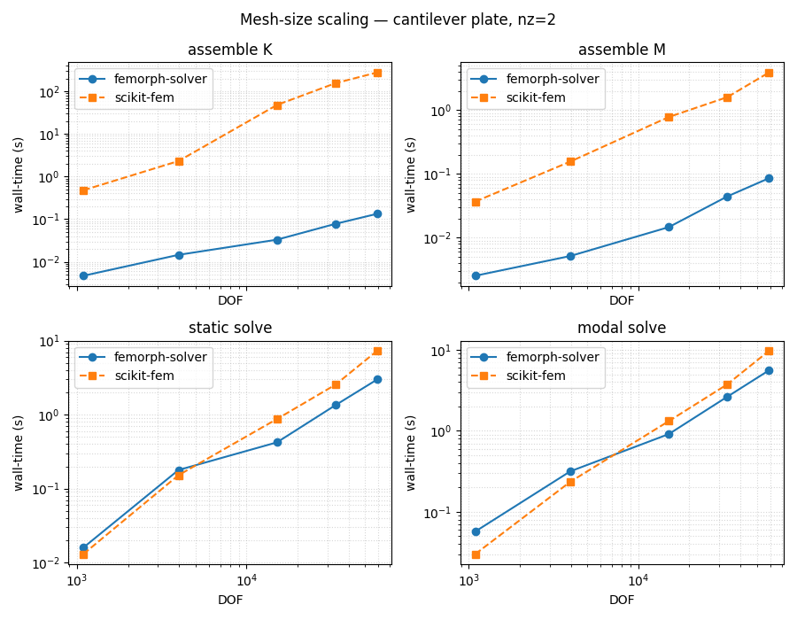
Scaling plot

One panel per stage (assemble K, assemble M, static, modal). Log-log so power-law scaling looks linear. The interesting reading is the slope: both solvers should scale O(n_dof) on assembly (roughly linear) and O(n_dof^{~1.3}) on the sparse direct solve.

import matplotlib.pyplot as plt  # noqa: E402

dofs = [m.n_dof for m in femorph_solver_runs]

fig, axes = plt.subplots(2, 2, figsize=(9, 7), sharex=True)
panels = [
    ("assemble K", "t_assemble_K_s", axes[0, 0]),
    ("assemble M", "t_assemble_M_s", axes[0, 1]),
    ("static solve", "t_static_s", axes[1, 0]),
    ("modal solve", "t_modal_s", axes[1, 1]),
]
for title, attr, ax in panels:
    ax.loglog(dofs, [getattr(m, attr) for m in femorph_solver_runs], "o-", label="femorph-solver")
    ax.loglog(dofs, [getattr(s, attr) for s in skf_runs], "s--", label="scikit-fem")
    ax.set_title(title)
    ax.set_xlabel("DOF")
    ax.set_ylabel("wall-time (s)")
    ax.grid(True, which="both", ls=":", alpha=0.5)
    ax.legend()
fig.suptitle(f"Mesh-size scaling — cantilever plate, nz={NZ}")
fig.tight_layout()
plt.show()