Note
Go to the end to download the full example code.
Single-hex uniaxial tension — Hooke’s law + Poisson check#
The smallest possible verification: a unit cube of isotropic linear elastic material under a uniform axial traction must reproduce 1-D Hooke’s law \(\sigma_{xx} = E\, \varepsilon_{xx}\) and Poisson contraction \(\varepsilon_{yy} = -\nu\, \varepsilon_{xx}\) to machine precision.
Reference: Hughes, T. J. R. The Finite Element Method, Dover, 2000, §2.7.
This gallery example drives the validation framework — the
PublishedValue carries the citation and the closed-form
formula; the acceptance test at the bottom mirrors the
regression guard in tests/validation/test_single_hex_uniaxial.py.
from __future__ import annotations

import numpy as np
import pyvista as pv

from femorph_solver.validation.problems import SingleHexUniaxial
Instantiate the benchmark#
Reports its published values in the order declared.
problem = SingleHexUniaxial()
print(f"benchmark: {problem.name}")
print(problem.description)
print()
for ref in problem.published_values:
    print(f"  {ref.name:18s}  {ref.value:+.6e} {ref.unit:3s}  [source: {ref.source}]")
    print(f"    formula: {ref.formula}")
benchmark: single_hex_uniaxial
Single 8-node hex under uniaxial tension — verifies 1-D Hooke's law and Poisson contraction to machine precision.

  tip_axial_disp      +5.000000e-06 m    [source: Hughes 2000 §2.7]
    formula: u_x(L) = sigma/E * L = P L / (E A)
  transverse_disp     -1.500000e-06 m    [source: Hughes 2000 §2.7]
    formula: u_y(L) = -nu eps_xx L
  sigma_xx_avg        +1.000000e+06 Pa   [source: Hughes 2000 §2.7]
    formula: sigma_xx = E eps_xx = P / A
Run the validation#
validate() builds the model, solves, and extracts each
published quantity. The default single-hex mesh is enough —
this problem is a direct consistency check, not a convergence
study.
results = problem.validate()
print("\ncomputed vs published:")
print(f"  {'quantity':<18s} {'computed':>14s} {'published':>14s}  {'rel err':>10s}  pass")
for r in results:
    pass_str = "✓" if r.passed else "✗"
    print(
        f"  {r.published.name:<18s} {r.computed:+14.6e} "
        f"{r.published.value:+14.6e}  "
        f"{r.rel_error * 100:+9.2e}%   {pass_str}"
    )
computed vs published:
  quantity                 computed      published     rel err  pass
  tip_axial_disp      +5.000000e-06  +5.000000e-06  +0.00e+00%   ✓
  transverse_disp     -1.500000e-06  -1.500000e-06  -1.41e-13%   ✓
  sigma_xx_avg        +1.000000e+06  +1.000000e+06  +0.00e+00%   ✓
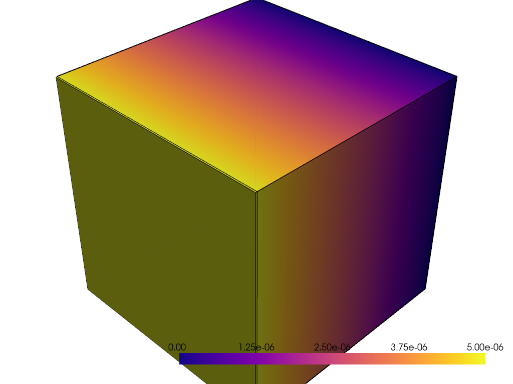
Visualise the deformed shape#
m = problem.build_model()
res = m.solve()
u = np.asarray(res.displacement).reshape(-1, 3)

# Exaggerate the displacement 1000× for visibility on the figure.
warped = m.grid.copy()
warped.points = m.grid.points + 1000.0 * u

plotter = pv.Plotter(off_screen=True)
plotter.add_mesh(m.grid, style="wireframe", color="black", line_width=1.5, label="undeformed")
plotter.add_mesh(warped, scalars=u[:, 0], show_edges=True, cmap="plasma", label="deformed (×1000)")
plotter.view_isometric()
plotter.camera.zoom(1.2)
plotter.show()
Acceptance#
Machine-precision pass is what Hooke’s law demands. Any regression here is either a constitutive-matrix / strain-kernel bug or a change in the solver residual; the framework surfaces both equally well.
for r in results:
    assert r.passed, (
        f"{r.published.name} drifted above the published tolerance: "
        f"rel_err={r.rel_error:.2e}, tol={r.published.tolerance:.2e}"
    )
Total running time of the script: (0 minutes 0.245 seconds)