Mesh-refinement convergence — cantilever Euler-Bernoulli#

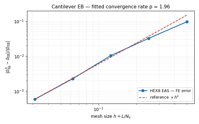
The textbook demonstration of FE convergence: for a fixed problem with a known closed form, refine the mesh and watch the discretisation error decrease at the asymptotic rate set by the element’s polynomial order. For the standard 8-node hex with enhanced-strain (Simo–Rifai) under a tip point load on a slender cantilever, the expected convergence rate in the energy / displacement norm is

\[\|u^{h} - u\| \;\sim\; C\, h^{p}, \qquad p = 2,\]

(Cook §6 + §6.3; Strang & Fix 2008 §3.7) — a quadratic decay of the tip-deflection error with the characteristic mesh length \(h\). Shear-locking-prone formulations (HEX8 plain Gauss without B-bar / EAS) fall short of this rate on thin-bending geometries, so this example is also a clean demonstration of why EAS is the right choice for solid-element plates and slender beams.

Implementation#

A unit-load cantilever of length \(L = 1\,\mathrm{m}\), square cross-section \(b = h = 0.1\,\mathrm{m}\), with one HEX8 element through the thickness in \(y\) and \(z\) and a refinement ladder in the axial direction \(N_x \in \{2, 4, 8, 16, 32\}\). At each refinement we fix the \(x = 0\) face in all three translations and apply a uniform tip force at the \(x = L\) face, then read the tip mid-surface UY against the Euler-Bernoulli closed form \(\delta = P L^{3} / (3 E I)\).

A least-squares fit to \(\log |\mathrm{error}|\) vs \(\log h\) recovers the asymptotic convergence rate \(p\).

References#

Cook, R. D., Malkus, D. S., Plesha, M. E., Witt, R. J. (2002) Concepts and Applications of Finite Element Analysis, 4th ed., Wiley, §6 (convergence of the FE method).
Strang, G. and Fix, G. (2008) An Analysis of the Finite Element Method, 2nd ed., Wellesley-Cambridge, §3.7 (a-priori error estimates for the Galerkin method).
Simo, J. C. and Rifai, M. S. (1990) “A class of mixed assumed strain methods …” International Journal for Numerical Methods in Engineering 29 (8), 1595–1638 (HEX8 EAS).
Bathe, K.-J. (2014) Finite Element Procedures, 2nd ed., §5.5 (a-posteriori error estimation), §11.7 (convergence rates for the discrete eigenvalue problem).

from __future__ import annotations

import math

import matplotlib.pyplot as plt
import numpy as np
import pyvista as pv

import femorph_solver
from femorph_solver import ELEMENTS

Problem data#

E = 2.0e11  # Pa
NU = 0.3
RHO = 7850.0
b = 0.1  # cross-section side [m]
A = b * b
I = b**4 / 12.0  # noqa: E741
L = 1.0  # span [m]
P_TOTAL = -5.0e3  # tip downward force [N]

delta_eb = P_TOTAL * L**3 / (3.0 * E * I)
print(f"L = {L} m, b = {b} m, EI = {E * I:.3e} N m^2")
print(f"δ_EB = P L^3 / (3 EI) = {delta_eb:.6e} m")


def run_one(nx: int) -> tuple[float, float]:
    """Return (h, |relative error|) for an Nx × 1 × 1 hex mesh."""
    xs = np.linspace(0.0, L, nx + 1)
    ys = np.linspace(0.0, b, 2)
    zs = np.linspace(0.0, b, 2)
    grid = pv.StructuredGrid(*np.meshgrid(xs, ys, zs, indexing="ij")).cast_to_unstructured_grid()

    m = femorph_solver.Model.from_grid(grid)
    m.assign(
        ELEMENTS.HEX8(integration="enhanced_strain"),
        material={"EX": E, "PRXY": NU, "DENS": RHO},
    )

    pts = np.asarray(m.grid.points)
    node_nums = np.asarray(m.grid.point_data["ansys_node_num"])
    fixed = node_nums[pts[:, 0] < 1e-9]
    m.fix(nodes=fixed.tolist(), dof="ALL")

    tip_mask = pts[:, 0] > L - 1e-9
    tip_nodes = node_nums[tip_mask]
    fz_per_node = P_TOTAL / len(tip_nodes)
    for nn in tip_nodes:
        m.apply_force(int(nn), fy=fz_per_node)

    res = m.solve()
    g = femorph_solver.io.static_result_to_grid(m, res)
    pts_g = np.asarray(g.points)
    tip_mask_g = pts_g[:, 0] > L - 1e-9
    uy_tip = float(g.point_data["displacement"][tip_mask_g, 1].mean())
    h = L / nx
    rel_err = abs(uy_tip - delta_eb) / abs(delta_eb)
    return h, rel_err

L = 1.0 m, b = 0.1 m, EI = 1.667e+06 N m^2
δ_EB = P L^3 / (3 EI) = -1.000000e-03 m

Asymptotic convergence rate via least-squares fit#

Drop the coarsest point (pre-asymptotic) and fit \(\log |\mathrm{err}| = -p\, \log h + c\) by ordinary linear regression on the log–log data.

log_h = np.log(np.asarray(hs[1:]))
log_err = np.log(np.asarray(errs[1:]))
slope, intercept = np.polyfit(log_h, log_err, 1)
p_estimated = float(slope)

print()
print(f"least-squares fit (Nx ≥ {nx_list[1]}): p ≈ {p_estimated:.3f}")
print("expected for HEX8 EAS bending response: p = 2")

# Allow some tolerance because the fit uses only 4 points and the
# coarsest of those is still slightly pre-asymptotic.
assert 1.5 < p_estimated, f"convergence rate {p_estimated:.3f} unexpectedly poor (< 1.5)"

least-squares fit (Nx ≥ 4): p ≈ 1.959
expected for HEX8 EAS bending response: p = 2

Render the convergence plot#

fig, ax = plt.subplots(1, 1, figsize=(6.4, 4.0))
ax.loglog(hs, errs, "o-", color="#1f77b4", lw=2, label="HEX8 EAS — FE error")

# Reference slope-2 line passing through the (h, err) at the finest
# mesh, for visual orientation.
h_ref = np.array([hs[0], hs[-1]])
err_ref_p2 = errs[-1] * (h_ref / hs[-1]) ** 2
ax.loglog(h_ref, err_ref_p2, "--", color="#d62728", lw=1.5, label=r"reference $\propto h^{2}$")

ax.set_xlabel(r"mesh size $h = L / N_x$")
ax.set_ylabel(r"$|\delta^{h}_{\mathrm{tip}} - \delta_{\mathrm{EB}}| / |\delta_{\mathrm{EB}}|$")
ax.set_title(
    f"Cantilever EB — fitted convergence rate p ≈ {p_estimated:.2f}",
    fontsize=11,
)
ax.legend(loc="lower right", fontsize=9)
ax.grid(True, which="both", ls=":", alpha=0.5)
fig.tight_layout()
fig.show()

Cantilever EB — fitted convergence rate p ≈ 1.96

Verify partition-of-unity: at every refinement the deflection stays the same sign as the analytical (negative for our downward load), and monotone-converges to it from below (HEX8 stiffens marginally vs. the analytical bending kinematics even with EAS — Cook §6.6 + §6.13).

assert all(e > 0 for e in errs), "errors must be positive (computed |·|)"
# Monotone decrease check (allow the last step to plateau within
# the asymptotic-floor noise).
for prev, nxt in zip(errs[:-1], errs[1:]):
    assert nxt < prev * 1.05, "error grew between successive refinements"
print()
print("OK — error decreases monotonically with refinement.")

OK — error decreases monotonically with refinement.

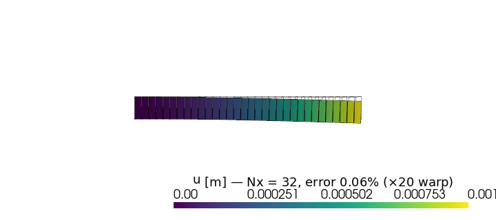
Render the deformed mesh at the finest resolution for visual orientation ————————————————————

xs = np.linspace(0.0, L, nx_list[-1] + 1)
ys = np.linspace(0.0, b, 2)
zs = np.linspace(0.0, b, 2)
grid = pv.StructuredGrid(*np.meshgrid(xs, ys, zs, indexing="ij")).cast_to_unstructured_grid()
m = femorph_solver.Model.from_grid(grid)
m.assign(ELEMENTS.HEX8(integration="enhanced_strain"), material={"EX": E, "PRXY": NU, "DENS": RHO})
pts = np.asarray(m.grid.points)
node_nums = np.asarray(m.grid.point_data["ansys_node_num"])
m.fix(nodes=node_nums[pts[:, 0] < 1e-9].tolist(), dof="ALL")
for nn in node_nums[pts[:, 0] > L - 1e-9]:
    m.apply_force(int(nn), fy=P_TOTAL / int((pts[:, 0] > L - 1e-9).sum()))
res = m.solve()
grid = femorph_solver.io.static_result_to_grid(m, res)

warp = grid.warp_by_vector("displacement", factor=20.0)
plotter = pv.Plotter(off_screen=True, window_size=(720, 320))
plotter.add_mesh(grid, style="wireframe", color="grey", opacity=0.4)
plotter.add_mesh(
    warp,
    scalars="displacement_magnitude",
    cmap="viridis",
    show_edges=True,
    scalar_bar_args={
        "title": f"|u| [m] — Nx = {nx_list[-1]}, error {errs[-1] * 100:.2f}% (×20 warp)"
    },
)
plotter.view_xy()
plotter.camera.zoom(1.05)
plotter.show()

# Compute the published-deflection magnitude for the title
print()
print(f"Published Euler-Bernoulli δ = {math.fabs(delta_eb):.4e} m")

example verify convergence cantilever eb

Published Euler-Bernoulli δ = 1.0000e-03 m

Total running time of the script: (0 minutes 0.518 seconds)

Gallery generated by Sphinx-Gallery