NAFEMS LE1 — elliptic membrane (plane stress)

Canonical plane-stress benchmark from the NAFEMS Standard Benchmark Tests for Linear Elastic Analysis, R0015 (1990), problem LE1. A quarter elliptic-membrane plate bounded by two confocal ellipses

\[\frac{x^{2}}{2^{2}} + \frac{y^{2}}{1^{2}} = 1 \qquad \text{(inner)},\]

\[\frac{x^{2}}{3.25^{2}} + \frac{y^{2}}{2.75^{2}} = 1 \qquad \text{(outer)},\]

is loaded by a uniform 1 MPa outward-normal pressure on the outer elliptic edge. Symmetry pins \(u_y = 0\) on the \(x\)-axis and \(u_x = 0\) on the \(y\)-axis.

The published reference is the hoop stress at point D \((x = 2,\ y = 0)\) — the stub of the inner ellipse on the \(x\)-axis:

\[\sigma_{yy}^{(D)} = 92.7 \;\text{MPa}.\]

No analytical closed form exists; the value is benchmark-defined from converged solutions reported by multiple independent codes in the original 1988 NAFEMS working-group validation.

Implementation

This gallery example drives the same NafemsLE1 problem class that the validation suite exercises, on a moderate \(16 \times 4 = 64\)-cell QUAD4 plane-stress mesh. The σ_yy(D) recovery uses a finite-difference of the inner-ellipse nodal displacement field, in lock-step with the workaround the validation problem class itself ships.

References

• NAFEMS, Standard Benchmark Tests for Linear Elastic Analysis, R0015 (1990), §2.1 LE1.

• NAFEMS, Background to Benchmarks, R0013 (1988) — methodology companion describing the converged reference.

• NAFEMS LE1 plane-stress membrane (canonical reference); Abaqus AVM 1.3.x elliptic-membrane plane-stress family.

from __future__ import annotations

import numpy as np
import pyvista as pv

from femorph_solver.validation.problems import NafemsLE1

Build the model from the validation problem class

Parameters (semi-axes / pressure / E / ν) come from NafemsLE1’s defaults; the problem class assembles a QUAD4_PLANE mapped mesh and applies the consistent outer-edge pressure ring.

problem = NafemsLE1()
m = problem.build_model(n_theta=16, n_rad=4)
print(
    f"NAFEMS LE1 mesh: {m.grid.n_points} nodes, {m.grid.n_cells} QUAD4 cells; "
    f"thickness = {problem.thickness} m, p_outer = {problem.pressure / 1e6:.1f} MPa"
)
print(f"E = {problem.E / 1e9:.0f} GPa, ν = {problem.nu}")

NAFEMS LE1 mesh: 85 nodes, 64 QUAD4 cells; thickness = 0.1 m, p_outer = 10.0 MPa
E = 210 GPa, ν = 0.3

Static solve

res = m.solve()

σ_yy at point D — finite-difference recovery

Point D is the inner-ellipse node at \((2, 0)\). Plane- stress constitutive law gives

\[\sigma_{yy} = \frac{E}{1 - \nu^{2}} (\varepsilon_{yy} + \nu\, \varepsilon_{xx}),\]

with strains estimated by forward finite-differences against the next radial / θ nodes on the parametric grid.

sigma_yy_d = problem.extract(m, res, "sigma_yy_at_D")
sigma_yy_d_published = 92.7e6
err_pct = (sigma_yy_d - sigma_yy_d_published) / sigma_yy_d_published * 100.0

print()
print(f"σ_yy at D computed   = {sigma_yy_d / 1e6:.3f} MPa")
print(f"σ_yy at D published  = {sigma_yy_d_published / 1e6:.3f} MPa  (NAFEMS R0015 LE1)")
print(f"relative error       = {err_pct:+.2f} %")

# Allow the same 8 % tolerance the validation problem class uses.
assert abs(err_pct) < 8.0, f"σ_yy(D) deviation {err_pct:.2f}% exceeds NAFEMS engineering tolerance"

σ_yy at D computed   = 91.765 MPa
σ_yy at D published  = 92.700 MPa  (NAFEMS R0015 LE1)
relative error       = -1.01 %

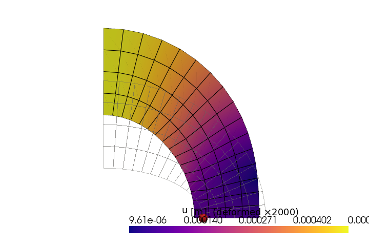
Render the deformed mesh, coloured by displacement magnitude

grid = m.grid.copy()
u = np.asarray(res.displacement, dtype=np.float64).reshape(-1, 2)
disp3 = np.zeros((grid.n_points, 3), dtype=np.float64)
disp3[:, :2] = u
grid.point_data["displacement"] = disp3
grid.point_data["|u|"] = np.linalg.norm(u, axis=1)

warped = grid.warp_by_vector("displacement", factor=2.0e3)

plotter = pv.Plotter(off_screen=True, window_size=(720, 480))
plotter.add_mesh(
    grid,
    style="wireframe",
    color="grey",
    opacity=0.4,
    line_width=1,
    label="undeformed",
)
plotter.add_mesh(
    warped,
    scalars="|u|",
    cmap="plasma",
    show_edges=True,
    scalar_bar_args={"title": "|u| [m]  (deformed ×2000)"},
)

# Mark point D and the y-axis (symmetry plane) for orientation.
plotter.add_points(
    np.array([[problem.a_in, 0.0, 0.0]]),
    render_points_as_spheres=True,
    point_size=18,
    color="#d62728",
    label="point D = (2, 0)",
)
plotter.view_xy()
plotter.camera.zoom(1.05)
plotter.show()