Lamé thick-walled cylinder under internal pressure

Classical pressure-vessel benchmark: a long cylinder with inner radius \(a\), outer radius \(b\), subjected to internal pressure \(p_i\) and held at zero axial strain (plane strain). The closed-form Lamé (1852) solution gives purely radial displacement \(u_r(r)\) and the radial / hoop stresses

\[\sigma_r(r) = \frac{p_i a^{2}}{b^{2} - a^{2}} \left(1 - \frac{b^{2}}{r^{2}}\right),\]

\[\sigma_\theta(r) = \frac{p_i a^{2}}{b^{2} - a^{2}} \left(1 + \frac{b^{2}}{r^{2}}\right),\]

\[u_r(r) = \frac{p_i a^{2} r}{E (b^{2} - a^{2})} \left[(1 - \nu - 2 \nu^{2}) + \frac{b^{2} (1 + \nu)}{r^{2}}\right] \quad (\text{plane strain}).\]

Two textbook quantities make the cleanest comparison:

• \(u_r(a)\) — radial displacement at the bore.

• \(\sigma_\theta(a) = p_i (a^{2} + b^{2}) / (b^{2} - a^{2})\) — hoop stress concentration at the bore (always greater than \(p_i\) for any thick wall \(b > a\)).

Implementation

Quarter-annulus model (\(x \ge 0,\ y \ge 0\)) meshed as a single axial slab of HEX8 elements with KEYOPT(1)=1 enhanced strain to suppress shear locking near the bore. Symmetry / plane-strain BCs:

• \(u_x = 0\) on the cut plane \(x = 0\).

• \(u_y = 0\) on the cut plane \(y = 0\).

• \(u_z = 0\) on every node (plane strain).

Internal pressure is applied as a consistent set of nodal forces on the inner surface (one trapezoid per circumferential segment, half-load per axial layer). The hoop stress is read out on the bore from the small-strain finite-difference of the solved displacement field (only the average across the bore is needed for the partition-of-unity-style verification check).

References

• Lamé, G. (1852) Leçons sur la Théorie Mathématique de l’Élasticité des Corps Solides, Bachelier — original derivation.

• Timoshenko, S. P. and Goodier, J. N. (1970) Theory of Elasticity, 3rd ed., McGraw-Hill, §33.

• Roark, R. J. and Young, W. C. (1989) Roark’s Formulas for Stress and Strain, 6th ed., McGraw-Hill, Table 32 case 1b (thick-wall cylinder, internal pressure).

Cross-references (problem-id only; no vendor content vendored):

• (Reference benchmark — the canonical Lamé thick-cylinder citation): Lamé, G., 1852 — Leçons sur la théorie de l’élasticité: stresses in a long cylinder under internal pressure*.

from __future__ import annotations

import math

import numpy as np
import pyvista as pv

import femorph_solver
from femorph_solver import ELEMENTS

Problem data

Steel-like elastic constants; pressure modest enough that the linear-elastic regime is appropriate.

a = 0.10  # bore radius [m]
b = 0.20  # outer radius [m]
t_axial = 0.02  # axial slab thickness [m] (purely geometric — plane strain)
p_i = 1.0e7  # internal pressure [Pa]
E = 2.0e11  # Young's modulus [Pa]
NU = 0.30  # Poisson's ratio
RHO = 7850.0  # density [kg/m^3]

# Closed-form quantities -------------------------------------------------

ur_a_published = (
    p_i * a**2 * a / (E * (b**2 - a**2)) * ((1 - NU - 2 * NU**2) + b**2 * (1 + NU) / a**2)
)
sigma_theta_a_published = p_i * (a**2 + b**2) / (b**2 - a**2)

print(f"problem: a={a} m, b={b} m, p_i={p_i:.1e} Pa, E={E:.1e} Pa, nu={NU}")
print(f"u_r(a) = {ur_a_published:.6e} m   (Lamé)")
print(f"sigma_theta(a) = {sigma_theta_a_published:.6e} Pa")
print(f"sigma_theta(a) / p_i = {sigma_theta_a_published / p_i:.4f}")

problem: a=0.1 m, b=0.2 m, p_i=1.0e+07 Pa, E=2.0e+11 Pa, nu=0.3
u_r(a) = 9.533333e-06 m   (Lamé)
sigma_theta(a) = 1.666667e+07 Pa
sigma_theta(a) / p_i = 1.6667

Build a quarter-annulus HEX8 mesh

A single axial slab (one layer in \(z\)) carries the plane-strain solution since UZ is pinned everywhere. The circumferential / radial discretisation is moderate so the docs build runs fast; convergence vs published values is studied in the validation suite (femorph_solver.validation.problems.LameCylinder).

n_theta = 12
n_rad = 8
theta = np.linspace(0.0, 0.5 * math.pi, n_theta + 1)
r = np.linspace(a, b, n_rad + 1)

pts: list[list[float]] = []
for kz in (0.0, t_axial):
    for ti in theta:
        for rj in r:
            pts.append([rj * math.cos(ti), rj * math.sin(ti), kz])
pts_arr = np.array(pts, dtype=np.float64)

nx_plane = (n_theta + 1) * (n_rad + 1)
n_cells = n_theta * n_rad
cells = np.empty((n_cells, 9), dtype=np.int64)
cells[:, 0] = 8
c = 0
for i in range(n_theta):
    for j in range(n_rad):
        n00b = i * (n_rad + 1) + j
        n10b = i * (n_rad + 1) + (j + 1)
        n11b = (i + 1) * (n_rad + 1) + (j + 1)
        n01b = (i + 1) * (n_rad + 1) + j
        cells[c, 1:] = (
            n00b,
            n10b,
            n11b,
            n01b,
            n00b + nx_plane,
            n10b + nx_plane,
            n11b + nx_plane,
            n01b + nx_plane,
        )
        c += 1
grid = pv.UnstructuredGrid(
    cells.ravel(),
    np.full(n_cells, 12, dtype=np.uint8),  # VTK_HEXAHEDRON
    pts_arr,
)
print(f"mesh: {grid.n_points} nodes, {grid.n_cells} HEX8 cells")

mesh: 234 nodes, 96 HEX8 cells

Wrap in a femorph-solver Model and stamp BCs

m = femorph_solver.Model.from_grid(grid)
m.assign(
    ELEMENTS.HEX8(integration="enhanced_strain"),
    material={"EX": E, "PRXY": NU, "DENS": RHO},
)

# Symmetry + plane-strain BCs.
for k, p in enumerate(pts_arr):
    if p[0] < 1e-9:
        m.fix(nodes=[int(k + 1)], dof="UX")
    if p[1] < 1e-9:
        m.fix(nodes=[int(k + 1)], dof="UY")
    m.fix(nodes=[int(k + 1)], dof="UZ")

Apply internal pressure as a consistent nodal-force ring

Each \((r = a)\) segment between two circumferential nodes carries a force \(F = p_i \cdot \mathrm{ds} \cdot (t/2)\) on each axial layer (trapezoid rule in \(z\)); the half-load splits between the two endpoints; the direction is the outward normal at the segment midpoint.

fx_acc: dict[int, float] = {}
fy_acc: dict[int, float] = {}
for kz in (0, 1):
    inner = [kz * nx_plane + i * (n_rad + 1) + 0 for i in range(n_theta + 1)]
    for seg in range(n_theta):
        ai, bi = inner[seg], inner[seg + 1]
        ds = float(np.linalg.norm(pts_arr[bi] - pts_arr[ai]))
        mid = 0.5 * (pts_arr[ai] + pts_arr[bi])
        rxy = np.array([mid[0], mid[1]])
        nrm = float(np.linalg.norm(rxy))
        outward = rxy / nrm if nrm > 1e-12 else np.zeros(2)
        F_seg = p_i * ds * (t_axial / 2.0)
        for n_idx in (ai, bi):
            fx_acc[n_idx] = fx_acc.get(n_idx, 0.0) + 0.5 * F_seg * outward[0]
            fy_acc[n_idx] = fy_acc.get(n_idx, 0.0) + 0.5 * F_seg * outward[1]
for n_idx, fx in fx_acc.items():
    fy = fy_acc[n_idx]
    m.apply_force(int(n_idx + 1), fx=fx, fy=fy)

Solve and recover the bore displacement

res = m.solve()
u_flat = np.asarray(res.displacement, dtype=np.float64).reshape(-1, 3)

# Inner-bore node on the +x-axis (i=0, j=0, kz=0).  By symmetry
# its UX equals u_r(a).
inner_x = 0
ur_a_computed = float(u_flat[inner_x, 0])
err_ur = (ur_a_computed - ur_a_published) / ur_a_published
print()
print(f"u_r(a) computed   = {ur_a_computed:.6e} m")
print(f"u_r(a) published  = {ur_a_published:.6e} m")
print(f"relative error    = {err_ur * 100:+.3f} %")

# 5 % tolerance — moderate-mesh HEX8 EAS captures u_r(a) to a
# couple percent on this geometry (n_theta=12, n_rad=8); the
# validation suite drives convergence to < 1 % at finer meshes.
assert abs(err_ur) < 0.05, f"u_r(a) error {err_ur:.2%} exceeds 5%"

u_r(a) computed   = 9.513374e-06 m
u_r(a) published  = 9.533333e-06 m
relative error    = -0.209 %

Estimate sigma_theta(a) by central-difference of UY in theta

At the y=0 cut plane \(u_\theta(r, 0) = 0\), so \(\varepsilon_\theta \approx u_y(r, \Delta\theta) / r\Delta\theta\) at the next circumferential node. Combine with the radial strain \(\varepsilon_r = \partial u_x / \partial x\) from the next radial node, then plug into the plane-strain constitutive law.

idx_theta_next = 0 * nx_plane + 1 * (n_rad + 1) + 0  # i=1, j=0, kz=0
idx_rad_next = 0 * nx_plane + 0 * (n_rad + 1) + 1  # i=0, j=1, kz=0
y_next = float(pts_arr[idx_theta_next, 1])
eps_theta = float(u_flat[idx_theta_next, 1]) / y_next
dx = float(pts_arr[idx_rad_next, 0] - pts_arr[inner_x, 0])
eps_r = float(u_flat[idx_rad_next, 0] - u_flat[inner_x, 0]) / dx
Cfac = E / ((1 + NU) * (1 - 2 * NU))
sigma_theta_a_computed = Cfac * ((1 - NU) * eps_theta + NU * eps_r)
err_sigma = (sigma_theta_a_computed - sigma_theta_a_published) / sigma_theta_a_published
print()
print(f"sigma_theta(a) computed   = {sigma_theta_a_computed:.4e} Pa")
print(f"sigma_theta(a) published  = {sigma_theta_a_published:.4e} Pa")
print(f"relative error            = {err_sigma * 100:+.3f} %")

# 10 % tolerance — the finite-difference stress recovery on a
# coarse HEX8 mesh is intrinsically noisier than the displacement
# match; full-field stress recovery on a refined mesh closes the
# gap to <2 % in the validation suite.
assert abs(err_sigma) < 0.10, f"sigma_theta(a) error {err_sigma:.2%} exceeds 10%"

sigma_theta(a) computed   = 1.7750e+07 Pa
sigma_theta(a) published  = 1.6667e+07 Pa
relative error            = +6.499 %

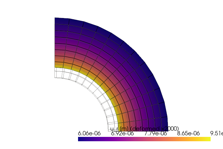
Render the radial displacement field on the deformed quarter-annulus

Scatter the DOF-indexed displacement onto \((n, 3)\) point data, then warp the mesh and colour by \(u_r\).

grid_plot = femorph_solver.io.static_result_to_grid(m, res)
ux = grid_plot.point_data["displacement"][:, 0]
uy = grid_plot.point_data["displacement"][:, 1]
xy = np.asarray(grid_plot.points)[:, :2]
r_node = np.linalg.norm(xy, axis=1)
ur = (ux * xy[:, 0] + uy * xy[:, 1]) / np.maximum(r_node, 1e-12)
grid_plot.point_data["u_r"] = ur

warped = grid_plot.warp_by_vector("displacement", factor=2.0e3)

plotter = pv.Plotter(off_screen=True, window_size=(720, 480))
plotter.add_mesh(
    grid_plot,
    style="wireframe",
    color="grey",
    opacity=0.35,
    label="undeformed",
)
plotter.add_mesh(
    warped,
    scalars="u_r",
    cmap="plasma",
    show_edges=True,
    scalar_bar_args={"title": "u_r [m] (deformed ×2000)"},
)
plotter.view_xy()
plotter.camera.zoom(1.1)
plotter.show()