Note
Go to the end to download the full example code.
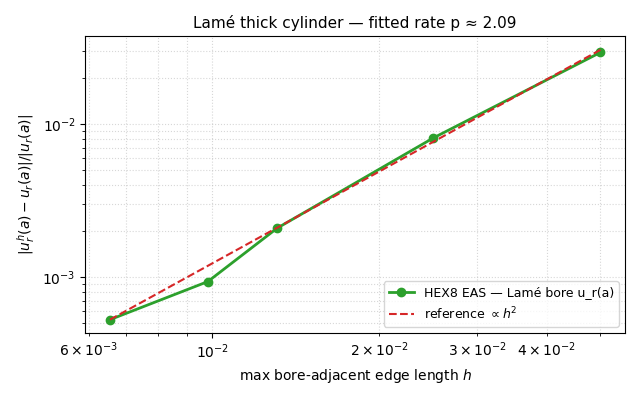
Mesh-refinement convergence — Lamé thick cylinder#
Companion to the Mesh-refinement convergence — cantilever Euler-Bernoulli beam study, this example shows the same \(O(h^{2})\) displacement-norm convergence rate on a 3D axisymmetric elasticity problem: the Lamé thick cylinder under internal pressure. Different physics (purely radial deformation, no bending), different element geometry (annular sector instead of beam-aspect prism), but the same Galerkin error theorem holds — Strang & Fix (2008) §3.7 promises \(\|u^{h} - u\|_{L^{2}} = O(h^{p+1})\) with \(p = 1\) for trilinear hex.
The bore radial displacement \(u_r(a) = (p_i\, a^{2}\, a / [E (b^{2} - a^{2})]) \cdot [(1 - \nu - 2\nu^{2}) + b^{2} (1 + \nu) / a^{2}]\) (Lamé 1852; Timoshenko & Goodier 1970 §33) gives the unambiguous reference value across every refinement.
Implementation#
Quarter-annulus HEX8 EAS plane-strain model (one axial layer) with a refinement ladder \((N_\theta, N_r) \in \{(4, 2), (8, 4), (12, 8), (16, 12), (24, 16)\}\). At each refinement we run the same internal- pressure-applied static solve as the Lamé thick-walled cylinder under internal pressure single-mesh example, then compare \(u_r(a)\) against the closed form. Mesh size \(h\) is taken as \(\max(\Delta\theta\, a, \Delta r)\) to characterise the largest element edge length on the bore- adjacent ring (where the gradient is steepest).
References#
Lamé, G. (1852) Leçons sur la Théorie Mathématique de l’Élasticité des Corps Solides, Bachelier — original derivation of the radial displacement.
Timoshenko, S. P. and Goodier, J. N. (1970) Theory of Elasticity, 3rd ed., McGraw-Hill, §33 (thick-walled cylinder).
Roark, R. J. and Young, W. C. (1989) Roark’s Formulas for Stress and Strain, 6th ed., McGraw-Hill, Table 32 case 1b.
Strang, G. and Fix, G. (2008) An Analysis of the Finite Element Method, 2nd ed., Wellesley-Cambridge, §3.7 (a-priori error estimates).
Cook, R. D., Malkus, D. S., Plesha, M. E., Witt, R. J. (2002) Concepts and Applications of Finite Element Analysis, 4th ed., Wiley, §6 (convergence).
Simo, J. C. and Rifai, M. S. (1990) “A class of mixed assumed strain methods …” International Journal for Numerical Methods in Engineering 29 (8), 1595–1638.
from __future__ import annotations

import math

import matplotlib.pyplot as plt
import numpy as np
import pyvista as pv

import femorph_solver
from femorph_solver import ELEMENTS
Problem data#
a = 0.10  # bore radius [m]
b = 0.20  # outer radius [m]
t_axial = 0.02
p_i = 1.0e7
E = 2.0e11
NU = 0.30
RHO = 7850.0

ur_a_published = (
    p_i * a**2 * a / (E * (b**2 - a**2)) * ((1 - NU - 2 * NU**2) + b**2 * (1 + NU) / a**2)
)
print(f"Lamé bore u_r(a) (Timoshenko & Goodier §33) = {ur_a_published * 1e6:.4f} µm")


def run_one(n_theta: int, n_rad: int) -> tuple[float, float]:
    """One quarter-annulus solve.  Returns (h, |relative error|)."""
    theta = np.linspace(0.0, 0.5 * math.pi, n_theta + 1)
    r = np.linspace(a, b, n_rad + 1)

    pts: list[list[float]] = []
    for kz in (0.0, t_axial):
        for ti in theta:
            for rj in r:
                pts.append([rj * math.cos(ti), rj * math.sin(ti), kz])
    pts_arr = np.array(pts, dtype=np.float64)

    nx_plane = (n_theta + 1) * (n_rad + 1)
    n_cells = n_theta * n_rad
    cells = np.empty((n_cells, 9), dtype=np.int64)
    cells[:, 0] = 8
    c = 0
    for i in range(n_theta):
        for j in range(n_rad):
            n00b = i * (n_rad + 1) + j
            n10b = i * (n_rad + 1) + (j + 1)
            n11b = (i + 1) * (n_rad + 1) + (j + 1)
            n01b = (i + 1) * (n_rad + 1) + j
            cells[c, 1:] = (
                n00b,
                n10b,
                n11b,
                n01b,
                n00b + nx_plane,
                n10b + nx_plane,
                n11b + nx_plane,
                n01b + nx_plane,
            )
            c += 1
    grid = pv.UnstructuredGrid(
        cells.ravel(),
        np.full(n_cells, 12, dtype=np.uint8),
        pts_arr,
    )

    m = femorph_solver.Model.from_grid(grid)
    m.assign(
        ELEMENTS.HEX8(integration="enhanced_strain"),
        material={"EX": E, "PRXY": NU, "DENS": RHO},
    )

    for k, p in enumerate(pts_arr):
        if p[0] < 1e-9:
            m.fix(nodes=[int(k + 1)], dof="UX")
        if p[1] < 1e-9:
            m.fix(nodes=[int(k + 1)], dof="UY")
        m.fix(nodes=[int(k + 1)], dof="UZ")

    fx_acc: dict[int, float] = {}
    fy_acc: dict[int, float] = {}
    for kz in (0, 1):
        inner = [kz * nx_plane + i * (n_rad + 1) + 0 for i in range(n_theta + 1)]
        for seg in range(n_theta):
            ai, bi = inner[seg], inner[seg + 1]
            ds = float(np.linalg.norm(pts_arr[bi] - pts_arr[ai]))
            mid = 0.5 * (pts_arr[ai] + pts_arr[bi])
            rxy = np.array([mid[0], mid[1]])
            nrm = float(np.linalg.norm(rxy))
            outward = rxy / nrm if nrm > 1e-12 else np.zeros(2)
            f_seg = p_i * ds * (t_axial / 2.0)
            for n_idx in (ai, bi):
                fx_acc[n_idx] = fx_acc.get(n_idx, 0.0) + 0.5 * f_seg * outward[0]
                fy_acc[n_idx] = fy_acc.get(n_idx, 0.0) + 0.5 * f_seg * outward[1]
    for n_idx, fx in fx_acc.items():
        fy = fy_acc[n_idx]
        m.apply_force(int(n_idx + 1), fx=fx, fy=fy)

    res = m.solve()
    u_flat = np.asarray(res.displacement, dtype=np.float64).reshape(-1, 3)
    inner_x = 0  # i=0, j=0, kz=0 sits at (a, 0, 0)
    ur_a_computed = float(u_flat[inner_x, 0])

    # Largest bore-adjacent edge.  Δθ · a (arc) vs Δr.
    h = max((0.5 * math.pi / n_theta) * a, (b - a) / n_rad)
    rel_err = abs(ur_a_computed - ur_a_published) / abs(ur_a_published)
    return h, rel_err
Lamé bore u_r(a) (Timoshenko & Goodier §33) = 9.5333 µm
Refinement ladder#
ladder = [(4, 2), (8, 4), (12, 8), (16, 12), (24, 16)]
hs: list[float] = []
errs: list[float] = []

print()
print(f"{'(N_θ, N_r)':>11}  {'h [m]':>10}  {'u_r(a) FE / pub':>16}  {'rel err':>10}")
print(f"{'-' * 11:>11}  {'-' * 10:>10}  {'-' * 16:>16}  {'-' * 10:>10}")
for n_th, n_r in ladder:
    h, err = run_one(n_th, n_r)
    hs.append(h)
    errs.append(err)
    print(f"({n_th:>3}, {n_r:>3})  {h:10.5f}  {(1 - err):>16.6f}  {err:10.4e}")
 (N_θ, N_r)       h [m]   u_r(a) FE / pub     rel err
-----------  ----------  ----------------  ----------
(  4,   2)     0.05000          0.970402  2.9598e-02
(  8,   4)     0.02500          0.991853  8.1472e-03
( 12,   8)     0.01309          0.997906  2.0936e-03
( 16,  12)     0.00982          0.999065  9.3544e-04
( 24,  16)     0.00654          0.999473  5.2717e-04
Asymptotic convergence rate#
log_h = np.log(np.asarray(hs[1:]))
log_err = np.log(np.asarray(errs[1:]))
slope, intercept = np.polyfit(log_h, log_err, 1)
p_estimated = float(slope)

print()
print(f"least-squares fit (skip first): rate p ≈ {p_estimated:.3f}")
print("expected for HEX8 EAS displacement norm (Strang & Fix §3.7): p = 2")

assert 1.4 < p_estimated, f"convergence rate {p_estimated:.3f} unexpectedly poor (< 1.4)"
least-squares fit (skip first): rate p ≈ 2.094
expected for HEX8 EAS displacement norm (Strang & Fix §3.7): p = 2
Render the convergence plot#
fig, ax = plt.subplots(1, 1, figsize=(6.4, 4.0))
ax.loglog(hs, errs, "o-", color="#2ca02c", lw=2, label="HEX8 EAS — Lamé bore u_r(a)")

h_ref = np.array([hs[0], hs[-1]])
err_ref_p2 = errs[-1] * (h_ref / hs[-1]) ** 2
ax.loglog(h_ref, err_ref_p2, "--", color="#d62728", lw=1.5, label=r"reference $\propto h^{2}$")

ax.set_xlabel(r"max bore-adjacent edge length $h$")
ax.set_ylabel(r"$|u_r^{h}(a) - u_r(a)| / |u_r(a)|$")
ax.set_title(
    f"Lamé thick cylinder — fitted rate p ≈ {p_estimated:.2f}",
    fontsize=11,
)
ax.legend(loc="lower right", fontsize=9)
ax.grid(True, which="both", ls=":", alpha=0.5)
fig.tight_layout()
fig.show()
Verify monotone decrease#
OK — error decreases monotonically with refinement.
Total running time of the script: (0 minutes 0.772 seconds)