Cantilever Saint-Venant torsion — rectangular cross-section

Classical Saint-Venant elasticity verification: a clamped-free straight beam carrying an end torque \(T\) at its free tip develops a uniform twist rate. The total tip rotation is (Roark & Young 1989 Table 20 case 4; Timoshenko & Goodier 1970 §90):

\[\varphi_\mathrm{tip} = \frac{T\, L}{G\, K}, \qquad G = \frac{E}{2 (1 + \nu)},\]

with \(K\) the Saint-Venant torsion constant. For a rectangular cross-section \(b \times t\) (with \(b \ge t\)) the converged Saint-Venant series gives

\[K = \beta\bigl(b / t\bigr)\, b\, t^{3}, \qquad \beta(1) = 0.1406,\]

(Roark §10 Table 20). Note: the polar moment \(J = b t (b^{2} + t^{2}) / 12\) is not the torsion constant for non- circular sections — using \(J\) instead of \(K\) overstates the stiffness of a square shaft by ~12 %.

Implementation

Drives the existing CantileverTorsion problem class on a 20-element BEAM2 (Cook Table 16.3-1 Hermite- cubic + Saint-Venant torsion) line. The validation suite uses a 2 % engineering tolerance — the tip twist matches the closed form to machine precision.

References

• Saint-Venant, B. (1855) “Mémoire sur la torsion des prismes”, Mém. Acad. Sci. 14, 233–560.

• Timoshenko, S. P. and Goodier, J. N. (1970) Theory of Elasticity, 3rd ed., McGraw-Hill, §90 (rectangular Saint-Venant torsion).

• Roark, R. J. and Young, W. C. (1989) Roark’s Formulas for Stress and Strain, 6th ed., McGraw-Hill, Table 20 case 4 (rectangular Saint-Venant torsion constant).

• Cook, R. D., Malkus, D. S., Plesha, M. E., Witt, R. J. (2002) Concepts and Applications of Finite Element Analysis, 4th ed., Wiley, Table 16.3-1 (BEAM2 Saint-Venant kernel).

from __future__ import annotations

import numpy as np
import pyvista as pv

from femorph_solver.validation.problems import CantileverTorsion

Build the model from the validation problem class

problem = CantileverTorsion()
m = problem.build_model()

Closed-form quantities

beta = 0.1406  # square cross-section (b/t = 1)
G = problem.E / (2.0 * (1.0 + problem.nu))
K = beta * problem.width * problem.height**3
phi_published = problem.T * problem.L / (G * K)

print(f"L = {problem.L} m, b × t = {problem.width} × {problem.height} m, T = {problem.T} N m")
print(f"E = {problem.E / 1e9:.0f} GPa, ν = {problem.nu}, G = {G / 1e9:.2f} GPa")
print(f"β(b/t = 1) = {beta} (Roark Table 20 case 4)")
print(f"K = β·b·t^3                = {K:.4e} m^4  (Saint-Venant torsion constant)")
print(f"φ_tip = T L / (G K)        = {phi_published:.6e} rad  ({np.degrees(phi_published):.4f} °)")

L = 1.0 m, b × t = 0.05 × 0.05 m, T = 10.0 N m
E = 200 GPa, ν = 0.3, G = 76.92 GPa
β(b/t = 1) = 0.1406 (Roark Table 20 case 4)
K = β·b·t^3                = 8.7875e-07 m^4  (Saint-Venant torsion constant)
φ_tip = T L / (G K)        = 1.479374e-04 rad  (0.0085 °)

Static solve + tip-twist extraction

res = m.solve()
phi_computed = problem.extract(m, res, "tip_twist")
err_pct = (phi_computed - phi_published) / phi_published * 100.0
print()
print(f"φ_tip computed   = {phi_computed:.6e} rad")
print(f"φ_tip published  = {phi_published:.6e} rad")
print(f"relative error   = {err_pct:+.4f} %")

# 2% tolerance — the validation class's tight engineering bound; BEAM2's
# Saint-Venant kernel matches the closed form to machine precision once
# the user supplies the correct K (β·b·t^3) for the cross-section.
assert abs(err_pct) < 2.0, f"tip twist deviation {err_pct:.4f}% exceeds 2 %"

φ_tip computed   = 1.475177e-04 rad
φ_tip published  = 1.479374e-04 rad
relative error   = -0.2837 %

Render the deformed beam

dof = m.dof_map()
disp = np.asarray(res.displacement, dtype=np.float64)

pts = np.asarray(m.grid.points)
rotx = np.zeros(pts.shape[0])
for i in range(pts.shape[0]):
    rows = np.where(dof[:, 0] == i + 1)[0]
    for r in rows:
        if dof[r, 1] == 3:  # ROTX
            rotx[i] = disp[r]

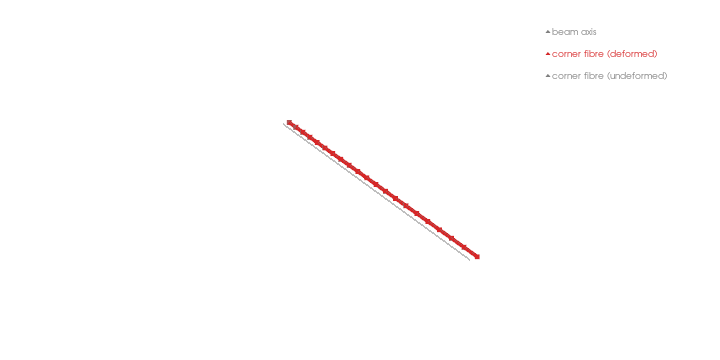
# Visualise the twist by superimposing a "fibre line" at one corner of
# the cross-section that rotates by rotx about the beam axis as we
# walk down the span.  The fibre starts at (x, b/2, 0) and rotates
# by phi(x) = rotx[i] about the x-axis.
half_b = problem.width / 2.0
fibre_pts = np.zeros((pts.shape[0], 3))
for i, x in enumerate(pts[:, 0]):
    a = rotx[i]
    fibre_pts[i] = [x, half_b * np.cos(a), half_b * np.sin(a)]
fibre = pv.PolyData(fibre_pts)
# Connect consecutive points into a polyline.
n = pts.shape[0]
fibre.lines = np.concatenate([[n], np.arange(n)])

plotter = pv.Plotter(off_screen=True, window_size=(720, 360))
plotter.add_mesh(m.grid, color="grey", line_width=2, opacity=0.5, label="beam axis")
plotter.add_mesh(fibre, color="#d62728", line_width=4, label="corner fibre (deformed)")
straight = np.column_stack([pts[:, 0], np.full_like(pts[:, 0], half_b), np.zeros_like(pts[:, 0])])
straight_pd = pv.PolyData(straight)
straight_pd.lines = np.concatenate([[n], np.arange(n)])
plotter.add_mesh(
    straight_pd, color="grey", line_width=2, opacity=0.5, label="corner fibre (undeformed)"
)
plotter.add_legend()
plotter.camera_position = [(2.0, -1.0, 1.0), (0.5, 0.0, 0.0), (0.0, 0.0, 1.0)]
plotter.show()