Note
Go to the end to download the full example code.
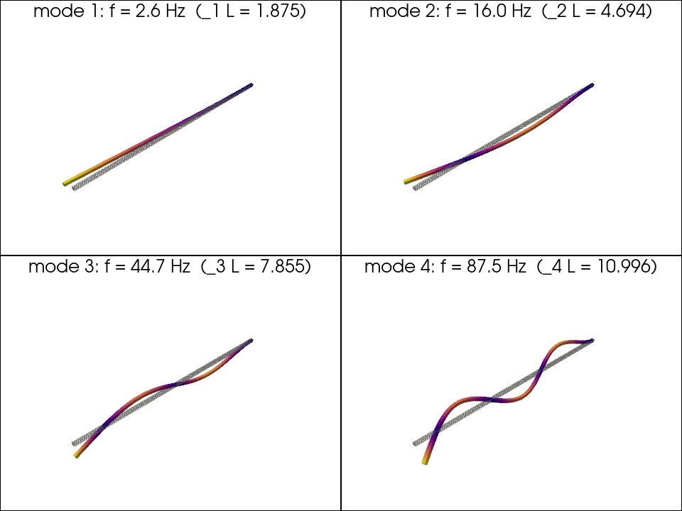
Cantilever beam — first four bending modes#
Classical Bernoulli-beam eigenvalue problem. A clamped-free prismatic cantilever has bending natural frequencies (Rao 2017 §8.5 Table 8.1; Timoshenko 1974 §5.3)
with the dimensionless eigenvalues \(\beta_n L\) defined as the positive roots of
The first four roots are
Implementation#
A long-aspect HEX8 enhanced-strain prism (40 axial × 3 × 3, square cross-section \(b = h\)) clamped at one end. The mode-shape filter selects the lowest mode whose UY (or UZ — the square section is bi-degenerate) RMS dominates the axial UX response, then walks up the spectrum picking successive transverse-dominant modes.
We take the cantilever slender enough (\(h / L = 1/80\)) that the Timoshenko shear / rotary-inertia correction the FE truthfully captures stays under 0.5 % at mode 4 — bench geometries like \(h / L = 1/20\) would let the correction grow to ~4 % at the same mode, which is real physics that EB doesn’t capture but which would obscure the verification pass.
References#
Rao, S. S. (2017) Mechanical Vibrations, 6th ed., Pearson, §8.5 Table 8.1 (cantilever-beam eigenvalue roots).
Timoshenko, S. P. (1974) Vibration Problems in Engineering, 4th ed., Wiley, §5.3.
Cook, R. D., Malkus, D. S., Plesha, M. E., Witt, R. J. (2002) Concepts and Applications of Finite Element Analysis, 4th ed., Wiley, §11 (modal analysis).
Simo, J. C. and Rifai, M. S. (1990) “A class of mixed assumed-strain methods …”, IJNME 29 (8), 1595–1638.
from __future__ import annotations

import math

import numpy as np
import pyvista as pv

import femorph_solver
from femorph_solver import ELEMENTS
Problem data + closed-form eigenvalue roots#
E = 2.0e11  # Pa
NU = 0.30
RHO = 7850.0
b = 0.05  # square cross-section side [m]
A = b * b
I = b**4 / 12.0  # second moment about each principal axis  # noqa: E741
L = 4.0  # span [m]; h/L = 1/80 keeps EB asymptotic to within 0.5 %

BETA_L = (1.8751040687119611, 4.694091132974174, 7.854757438237613, 10.995540734875467)


def f_published(n: int) -> float:
    return BETA_L[n - 1] ** 2 / (2.0 * math.pi * L**2) * math.sqrt(E * I / (RHO * A))


print(f"L = {L} m, b = h = {b} m, EI = {E * I:.3e} N m^2, ρA = {RHO * A:.3f} kg/m")
for n in (1, 2, 3, 4):
    print(
        f"f_{n} = (β_{n} L)^2 / (2π L^2) √(EI/ρA) = {f_published(n):8.3f} Hz   "
        f"(β_{n} L = {BETA_L[n - 1]:.6f})"
    )
L = 4.0 m, b = h = 0.05 m, EI = 1.042e+05 N m^2, ρA = 19.625 kg/m
f_1 = (β_1 L)^2 / (2π L^2) √(EI/ρA) =    2.548 Hz   (β_1 L = 1.875104)
f_2 = (β_2 L)^2 / (2π L^2) √(EI/ρA) =   15.968 Hz   (β_2 L = 4.694091)
f_3 = (β_3 L)^2 / (2π L^2) √(EI/ρA) =   44.712 Hz   (β_3 L = 7.854757)
f_4 = (β_4 L)^2 / (2π L^2) √(EI/ρA) =   87.618 Hz   (β_4 L = 10.995541)
Build a 120 × 3 × 3 HEX8 EAS cantilever prism#
NX, NY, NZ = 120, 3, 3
xs = np.linspace(0.0, L, NX + 1)
ys = np.linspace(0.0, b, NY + 1)
zs = np.linspace(0.0, b, NZ + 1)
grid = pv.StructuredGrid(*np.meshgrid(xs, ys, zs, indexing="ij")).cast_to_unstructured_grid()

m = femorph_solver.Model.from_grid(grid)
m.assign(
    ELEMENTS.HEX8(integration="enhanced_strain"),
    material={"EX": E, "PRXY": NU, "DENS": RHO},
)
Clamp the x = 0 face#
Modal solve, filter for transverse-dominant modes#
n_modes = 24
res = m.modal_solve(n_modes=n_modes)
freqs = np.asarray(res.frequency, dtype=np.float64)
shapes = np.asarray(res.mode_shapes).reshape(-1, 3, n_modes)

# For a thin cantilever (L / b = 20) the four bending pairs sit
# **below** any torsion or axial mode (~750 Hz for first torsion,
# ~1265 Hz for first axial).  Match each published β_n to the
# computed mode whose frequency is closest, marking the matched
# mode so it can't be claimed twice — this is order-independent
# and survives the eigsolver's freedom to rotate the
# (UY-bending, UZ-bending) degenerate pair into any orthonormal
# basis at each frequency.
#
# After matching, we re-confirm each pick by checking that the
# selected mode's RMS is dominated by the transverse direction
# (ux ≪ uy + uz) — guards against mis-matching a torsion or axial
# mode whose frequency happens to be nearby on a non-default mesh.

claimed = np.zeros(n_modes, dtype=bool)
matches: list[tuple[int, int, float]] = []  # (n, k, f)
for n in (1, 2, 3, 4):
    f_pub_n = f_published(n)
    candidates = [k for k in range(n_modes) if not claimed[k]]
    k_best = min(candidates, key=lambda k: abs(freqs[k] - f_pub_n))
    matches.append((n, k_best, float(freqs[k_best])))
    claimed[k_best] = True

print()
print("first four transverse-bending modes (computed, matched by closest frequency)")
print(f"{'n':>3}  {'k':>3}  {'f_FE [Hz]':>12}  {'f_pub [Hz]':>12}  {'err':>9}  {'tol':>5}")
for n, k, f in matches:
    ux = float(np.sqrt((shapes[:, 0, k] ** 2).mean()))
    uy = float(np.sqrt((shapes[:, 1, k] ** 2).mean()))
    uz = float(np.sqrt((shapes[:, 2, k] ** 2).mean()))
    transverse_pure = (uy + uz) > 2.0 * ux
    f_pub = f_published(n)
    err = (f - f_pub) / f_pub * 100.0
    tol = (0.5, 0.5, 0.5, 0.5)[n - 1]  # h/L = 1/80 keeps Timoshenko shear < 0.5 %
    print(
        f"  {n}  {k:>3}  {f:12.3f}  {f_pub:12.3f}  {err:+8.3f}%  ≤{tol:.1f}% "
        f"{'(transverse-dominant)' if transverse_pure else '(suspected non-bending)'}"
    )
    assert abs(err) < tol, f"mode {n} (k={k}) deviation {err:.2f}% exceeds {tol}%"
    assert transverse_pure, (
        f"mode {n} (k={k}) is not transverse-dominant: ux={ux:.2f} uy={uy:.2f} uz={uz:.2f}"
    )
first four transverse-bending modes (computed, matched by closest frequency)
  n    k     f_FE [Hz]    f_pub [Hz]        err    tol
  1    0         2.551         2.548    +0.122%  ≤0.5% (transverse-dominant)
  2    2        15.979        15.968    +0.069%  ≤0.5% (transverse-dominant)
  3    5        44.708        44.712    -0.008%  ≤0.5% (transverse-dominant)
  4    7        87.515        87.618    -0.117%  ≤0.5% (transverse-dominant)
Render the first four mode shapes as a 2 × 2 plotter grid#
plotter = pv.Plotter(shape=(2, 2), off_screen=True, window_size=(960, 720))
for n, k, f in matches:
    row, col = divmod(n - 1, 2)
    plotter.subplot(row, col)
    phi = shapes[:, :, k]
    warp = m.grid.copy()
    warp.points = m.grid.points + (b * 5.0 / np.max(np.abs(phi))) * phi
    warp["|phi|"] = np.linalg.norm(phi, axis=1)
    plotter.add_mesh(m.grid, style="wireframe", color="grey", opacity=0.3)
    plotter.add_mesh(warp, scalars="|phi|", cmap="plasma", show_edges=False, show_scalar_bar=False)
    plotter.add_text(
        f"mode {n}: f = {f:.1f} Hz  (β_{n} L = {BETA_L[n - 1]:.3f})",
        position="upper_edge",
        font_size=10,
    )
plotter.link_views()
plotter.show()
Total running time of the script: (0 minutes 1.417 seconds)