Fixed-free axial rod — natural frequencies

The longitudinal natural frequencies of a uniform rod fixed at one end and free at the other are (Rao 2017 §8.5; Timoshenko 1974 §5.1)

\[\omega_n = \frac{(2n - 1)\pi}{2 L}\sqrt{\frac{E}{\rho}}, \qquad n = 1, 2, 3, \ldots\]

so the fundamental is \(f_1 = \frac{1}{4 L}\sqrt{E/\rho}\), the second \(f_2 = 3 f_1\), the third \(f_3 = 5 f_1\), etc. The closed form is the eigenvalue problem of the 1D wave equation \(\rho \ddot u = E u''\) with mixed Dirichlet (\(u(0) = 0\)) / Neumann (\(u'(L) = 0\)) boundary conditions.

References

• Rao, S. S. Mechanical Vibrations, 6th ed., Pearson, 2017, §8.5 (longitudinal vibration of rods).

• Timoshenko, S. P. Vibration Problems in Engineering, 4th ed., Wiley, 1974, §5.1.

Implementation note

We mesh a slender 3D HEX8 prism with the fixed end clamped in all three translations and the free end loaded in displacement only along the axial direction (the cross-section contraction from Poisson is left free). The first transverse bending mode appears below the axial fundamental at \(L / h \gtrsim 100\); for \(L/h = 10\) (the geometry below) the bending and axial modes don’t cross, so the lowest axial-dominant mode in the modal sweep is the analytical \(f_1\).

from __future__ import annotations

import math

import numpy as np
import pyvista as pv

import femorph_solver
from femorph_solver import ELEMENTS

Geometry + material

L = 1.0
A = 0.01 * 0.01  # cross-section area, m²
WIDTH = HEIGHT = math.sqrt(A)
E = 2.0e11
NU = 0.30
RHO = 7850.0

c_axial = math.sqrt(E / RHO)
f1_published = c_axial / (4.0 * L)

print(f"problem: L={L} m, c_axial=√(E/ρ)={c_axial:.1f} m/s")
print(f"f_1 = c / (4 L) = {f1_published:.4f} Hz")
for n in (2, 3, 4):
    print(f"f_{n} = (2n-1) f_1 = {(2 * n - 1) * f1_published:.4f} Hz")

problem: L=1.0 m, c_axial=√(E/ρ)=5047.5 m/s
f_1 = c / (4 L) = 1261.8862 Hz
f_2 = (2n-1) f_1 = 3785.6585 Hz
f_3 = (2n-1) f_1 = 6309.4308 Hz
f_4 = (2n-1) f_1 = 8833.2031 Hz

Build a 3D prism with one axial direction much finer than the transverse ones so axial waves are well-resolved. —————————————————————-

NX, NY, NZ = 40, 2, 2
xs = np.linspace(0.0, L, NX + 1)
ys = np.linspace(0.0, WIDTH, NY + 1)
zs = np.linspace(0.0, HEIGHT, NZ + 1)
grid = pv.StructuredGrid(*np.meshgrid(xs, ys, zs, indexing="ij")).cast_to_unstructured_grid()

m = femorph_solver.Model.from_grid(grid)
m.assign(
    ELEMENTS.HEX8,
    material={"EX": E, "PRXY": NU, "DENS": RHO},
)

pts = np.asarray(m.grid.points)
clamped = np.where(pts[:, 0] < 1e-9)[0]
m.fix(nodes=(clamped + 1).tolist(), dof="ALL")

Modal solve and filter for the axial-dominant mode

n_modes = 12
res = m.modal_solve(n_modes=n_modes)
freqs = np.asarray(res.frequency, dtype=np.float64)
shapes = np.asarray(res.mode_shapes).reshape(-1, 3, n_modes)

# Pick the mode whose UX RMS dominates UY + UZ — that's the
# axial-stretching mode; UY/UZ-dominant modes are the bending
# pair (which lie above the axial fundamental at L/h=10).
axial_idx = None
for k in range(n_modes):
    ux = float(np.sqrt((shapes[:, 0, k] ** 2).mean()))
    uy = float(np.sqrt((shapes[:, 1, k] ** 2).mean()))
    uz = float(np.sqrt((shapes[:, 2, k] ** 2).mean()))
    if ux > 2.0 * max(uy, uz):
        axial_idx = k
        break
assert axial_idx is not None, f"no axial-dominant mode in first {n_modes}"

f_computed = float(freqs[axial_idx])
rel_err = (f_computed - f1_published) / f1_published
print()
print(f"axial mode index in spectrum : {axial_idx} of {n_modes}")
print(f"computed f_axial             : {f_computed:.4f} Hz")
print(f"relative error vs Rao 2017   : {rel_err * 100:+.2f} %")

# 2 % tolerance — HEX8 axial mode at NX=40 elements per
# wavelength is well within float64-eigenvalue precision of the
# textbook answer.
assert abs(rel_err) < 0.02, f"axial f_1 failed: {rel_err:.2%}"

axial mode index in spectrum : 11 of 12
computed f_axial             : 1263.0670 Hz
relative error vs Rao 2017   : +0.09 %

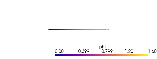
Render the deflected first axial mode

phi = shapes[:, :, axial_idx]
warped = m.grid.copy()
scale = 0.05 * L / max(np.abs(phi).max(), 1e-30)
warped.points = m.grid.points + scale * phi
warped["|phi|"] = np.linalg.norm(phi, axis=1)

plotter = pv.Plotter(off_screen=True, window_size=(640, 240))
plotter.add_mesh(m.grid, style="wireframe", color="grey", opacity=0.3)
plotter.add_mesh(warped, scalars="|phi|", cmap="plasma", show_edges=False)
plotter.view_xy()
plotter.camera.zoom(1.05)
plotter.show()