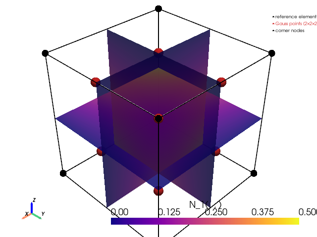
HEX8 reference geometry — nodes, shape functions, Gauss points

Renders the 8-node trilinear hexahedron’s reference element \(\hat\Omega = [-1, 1]^3\) with three layers of annotation:

1. Corner nodes with their natural-coordinate triplets \((\xi_i, \eta_i, \zeta_i) \in \{-1, +1\}^3\).

2. Trilinear Lagrange shape functions

   \[N_i(\xi, \eta, \zeta) = \tfrac{1}{8}(1 + \xi_i\xi)(1 + \eta_i\eta)(1 + \zeta_i\zeta), \qquad i = 1, \ldots, 8,\]

   evaluated on a sampling lattice and visualised by colouring the reference cube faces with \(N_1(\xi, \eta, \zeta)\).

3. 2×2×2 Gauss-Legendre integration points at \((\xi, \eta, \zeta) \in \{-1, +1\}/\sqrt{3}\), used by the stiffness and consistent-mass integrals on this element.

References

• Hughes, T. J. R. (2000) The Finite Element Method — Linear Static and Dynamic Finite Element Analysis, Dover, §3.1 (trilinear shape functions); §3.10 (Gauss-Legendre quadrature).

• Cook, R. D., Malkus, D. S., Plesha, M. E., Witt, R. J. (2002) Concepts and Applications of Finite Element Analysis, 4th ed., Wiley, §6.2.

• Zienkiewicz, O. C. and Taylor, R. L. (2013) The Finite Element Method: Its Basis and Fundamentals, 7th ed., Butterworth- Heinemann, §6.

Implementation: femorph_solver.elements.hex8.Hex8.

from __future__ import annotations

import numpy as np
import pyvista as pv

Reference cube as a single-cell pyvista UnstructuredGrid

Native HEX8 corner ordering (ξ, η, ζ) ∈ {-1, +1}^3 follows the standard isoparametric convention — VTK_HEXAHEDRON’s node order matches it, so we author the geometry once and visualise directly.

corners = np.array(
    [
        [-1, -1, -1],
        [+1, -1, -1],
        [+1, +1, -1],
        [-1, +1, -1],
        [-1, -1, +1],
        [+1, -1, +1],
        [+1, +1, +1],
        [-1, +1, +1],
    ],
    dtype=float,
)
cells = np.hstack([[8], np.arange(8, dtype=np.int64)])
cell_types = np.array([pv.CellType.HEXAHEDRON], dtype=np.uint8)
ref_cube = pv.UnstructuredGrid(cells, cell_types, corners)

Shape function \(N_1\) over a sampling lattice

Sample \(N_1(\xi, \eta, \zeta) = \tfrac18 (1 - \xi)(1 - \eta) (1 - \zeta)\) on a 21^3 lattice and store as a StructuredGrid point array. Slicing through the volume gives 2D contour-friendly views.

n = 21
xi = eta = zeta = np.linspace(-1.0, 1.0, n)
XI, ETA, ZETA = np.meshgrid(xi, eta, zeta, indexing="ij")
N1 = (1.0 - XI) * (1.0 - ETA) * (1.0 - ZETA) / 8.0
sample = pv.StructuredGrid(XI, ETA, ZETA)
sample["N_1"] = N1.ravel(order="F")

2×2×2 Gauss-Legendre integration points

g = 1.0 / np.sqrt(3.0)
gauss = np.array(
    [(a, b, c) for a in (-g, +g) for b in (-g, +g) for c in (-g, +g)],
    dtype=float,
)
gauss_pd = pv.PolyData(gauss)
gauss_pd["weight"] = np.full(len(gauss), 1.0)

Render the figure

Three glyphs share the same scene: the reference-cube wireframe (black), an \(N_1\) slice through the centre (warm colormap), and the eight Gauss points as red spheres.

plotter = pv.Plotter(off_screen=True, window_size=(640, 480))
plotter.add_mesh(
    ref_cube,
    style="wireframe",
    color="black",
    line_width=2,
    label="reference element",
)
slc = sample.slice_orthogonal(x=0.0, y=0.0, z=0.0)
plotter.add_mesh(
    slc,
    scalars="N_1",
    cmap="plasma",
    show_edges=False,
    opacity=0.85,
    scalar_bar_args={"title": "N_1(ξ, η, ζ)"},
)
plotter.add_points(
    gauss,
    render_points_as_spheres=True,
    point_size=20,
    color="#d62728",
    label="Gauss points (2×2×2)",
)
# Corner-node spheres
plotter.add_points(
    corners,
    render_points_as_spheres=True,
    point_size=14,
    color="black",
    label="corner nodes",
)
plotter.add_axes(line_width=4, color="black")
plotter.view_isometric()
plotter.camera.zoom(1.1)
plotter.add_legend(face=None, size=(0.18, 0.10), bcolor="white")
plotter.show()

Verify the partition of unity

At any point inside \(\hat\Omega\) the eight shape functions must sum to one. Sampling \(N_i(\xi_q, \eta_q, \zeta_q)\) at every Gauss point and asserting \(\sum_i N_i = 1\) is a minimal sanity check — failure would point to a typo in the kernel’s shape-function evaluation.

xi_i, eta_i, zeta_i = corners.T
sums = np.array(
    [
        sum(
            (1 + xi_i * a) * (1 + eta_i * b) * (1 + zeta_i * c) / 8.0
            for a, b, c in [(g[0], g[1], g[2])]
        ).sum()
        for g in gauss
    ]
)
print("partition-of-unity Σ N_i at each Gauss point:")
for q, s in zip(gauss, sums, strict=True):
    print(f"  ξ={q[0]:+.4f}  η={q[1]:+.4f}  ζ={q[2]:+.4f}  Σ={s:.15f}")
np.testing.assert_allclose(sums, 1.0, atol=1.0e-14)
print("OK — all 8 shape functions sum to 1 at every Gauss point.")

partition-of-unity Σ N_i at each Gauss point:
  ξ=-0.5774  η=-0.5774  ζ=-0.5774  Σ=1.000000000000000
  ξ=-0.5774  η=-0.5774  ζ=+0.5774  Σ=1.000000000000000
  ξ=-0.5774  η=+0.5774  ζ=-0.5774  Σ=1.000000000000000
  ξ=-0.5774  η=+0.5774  ζ=+0.5774  Σ=1.000000000000000
  ξ=+0.5774  η=-0.5774  ζ=-0.5774  Σ=1.000000000000000
  ξ=+0.5774  η=-0.5774  ζ=+0.5774  Σ=1.000000000000000
  ξ=+0.5774  η=+0.5774  ζ=-0.5774  Σ=1.000000000000000
  ξ=+0.5774  η=+0.5774  ζ=+0.5774  Σ=1.000000000000000
OK — all 8 shape functions sum to 1 at every Gauss point.