POINT_MASS — single-DOF spring-mass oscillator

Two nodes connected by a SPRING element. A POINT_MASS element sits on the free node. The first modal frequency is compared to the textbook SDOF result ω = √(k / m).

from __future__ import annotations

import numpy as np
import pyvista as pv
from vtkmodules.util.vtkConstants import VTK_LINE, VTK_VERTEX

import femorph_solver
from femorph_solver import ELEMENTS

Problem data

k = 1 kN/m, m = 0.25 kg → ω = √(4000) ≈ 63.2456 rad/s (f ≈ 10.065 Hz).

k = 1000.0
mass = 0.25
omega_expected = np.sqrt(k / mass)
f_expected = omega_expected / (2.0 * np.pi)

Build the model

Two element types: SPRING (spring, TYPE 1) and POINT_MASS (point mass, TYPE 2). Each gets its own REAL set. The grid carries per-cell ansys_elem_type_num / ansys_real_constant arrays that pin the kernel + real-set down element-by-element — the same routing legacy APDL uses but stamped on the grid up front.

points = np.array([[0.0, 0.0, 0.0], [1.0, 0.0, 0.0]], dtype=np.float64)
cells = np.array([2, 0, 1, 1, 1], dtype=np.int64)  # VTK_LINE(0,1) + VTK_VERTEX(1)
cell_types = np.array([VTK_LINE, VTK_VERTEX], dtype=np.uint8)
grid = pv.UnstructuredGrid(cells, cell_types, points)
grid.cell_data["ansys_elem_type_num"] = np.array([1, 2], dtype=np.int32)
grid.cell_data["ansys_real_constant"] = np.array([1, 2], dtype=np.int32)

mdl = femorph_solver.Model.from_grid(grid)
mdl.assign(ELEMENTS.SPRING, real=(k,), et_id=1, real_id=1)
mdl.assign(ELEMENTS.POINT_MASS, real=(mass,), et_id=2, real_id=2)

mdl.fix(nodes=[1], dof="ALL")  # clamp the spring base
mdl.fix(nodes=[2], dof="UY")  # kill transverse rigid-body modes
mdl.fix(nodes=[2], dof="UZ")
m = mdl  # alias preserves later references in this script

Modal solve + analytical comparison

Only one physical DOF is free (UX at node 2). modal_solve returns a single positive eigenvalue whose square root is ω.

res = m.modal_solve(n_modes=1)
omega_computed = float(np.sqrt(res.omega_sq[0]))
f_computed = float(res.frequency[0])

print(f"Expected ω = {omega_expected:.6f} rad/s, f = {f_expected:.6f} Hz")
print(f"Computed ω = {omega_computed:.6f} rad/s, f = {f_computed:.6f} Hz")
assert np.isclose(omega_computed, omega_expected, rtol=1e-10)

Expected ω = 63.245553 rad/s, f = 10.065842 Hz
Computed ω = 63.245553 rad/s, f = 10.065842 Hz

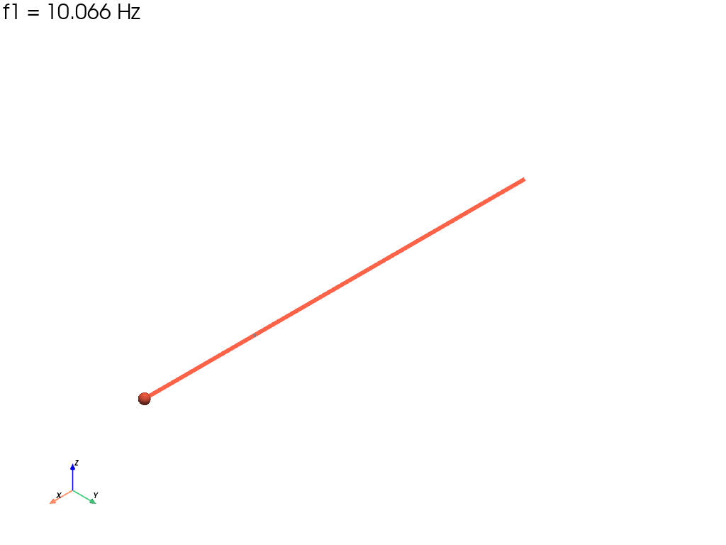
Plot the mode shape

Dilate the mode shape for visualisation. With POINT_MASS being a single-node element the mesh contains a VTK_LINE (the spring) and a VTK_VERTEX (the mass) — pyvista happily draws the combined unstructured grid.

dof = m.dof_map()
mode = res.mode_shapes[:, 0]
grid = m.grid.copy()
displacement = np.zeros((grid.n_points, 3), dtype=np.float64)
for i, nn in enumerate(grid.point_data["ansys_node_num"]):
    rows = np.where(dof[:, 0] == int(nn))[0]
    for r in rows:
        displacement[i, int(dof[r, 1])] = mode[r]
# Scale so the peak is 0.3 m for clarity.
peak = float(np.max(np.abs(displacement))) or 1.0
displacement *= 0.3 / peak
grid.point_data["mode1"] = displacement

warped = grid.warp_by_vector("mode1", factor=1.0)
plotter = pv.Plotter(off_screen=True)
plotter.add_mesh(grid, style="wireframe", color="gray", line_width=3)
plotter.add_mesh(
    warped,
    color="tomato",
    line_width=6,
    render_points_as_spheres=True,
    point_size=18,
)
plotter.add_text(f"f1 = {f_computed:.3f} Hz", font_size=12)
plotter.add_axes()
plotter.show()