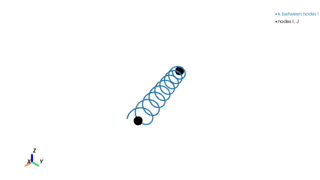
SPRING — 2-node longitudinal spring stiffness

The 2-node 3D longitudinal spring carries an axial-only stiffness \(k\) between two nodes connected by a unit direction vector \(\hat d = (l, m, n)\). No mass. Three translational DOFs per node, 6 DOFs per element.

Local axial-only stiffness on the natural coordinate \(s \in [-1, +1]\):

\[\begin{split}K_\text{local} = k \begin{bmatrix} +1 & -1 \\ -1 & +1 \end{bmatrix},\end{split}\]

embedded in 3D via the direction-cosine block \(T = \hat d\, \hat d^{\!\top}\):

\[\begin{split}K_e = k \begin{bmatrix} +T & -T \\ -T & +T \end{bmatrix}.\end{split}\]

References

• Cook, R. D., Malkus, D. S., Plesha, M. E., Witt, R. J. (2002) Concepts and Applications of Finite Element Analysis, 4th ed., Wiley, §3.2.

• Przemieniecki, J. S. (1968) Theory of Matrix Structural Analysis, McGraw-Hill, §3.

Implementation: femorph_solver.elements.spring.Spring.

from __future__ import annotations

import numpy as np
import pyvista as pv

2-node spring, drawn along an arbitrary direction

# Pick a non-axial direction so the figure shows the rotation
# from local to global axis.
end_a = np.array([0.0, 0.0, 0.0])
end_b = np.array([1.0, 0.6, 0.4])
length = float(np.linalg.norm(end_b - end_a))
direction = (end_b - end_a) / length

# Spring as a coil polyline along the I→J axis.
n_turns = 8
n_pts = 240
t = np.linspace(0.0, 1.0, n_pts)
axial = end_a + np.outer(t, end_b - end_a)
# Build two perpendicular vectors to ``direction`` for the coil radius.
ref = np.array([0.0, 0.0, 1.0]) if abs(direction[2]) < 0.9 else np.array([1.0, 0.0, 0.0])
e1 = np.cross(direction, ref)
e1 /= np.linalg.norm(e1)
e2 = np.cross(direction, e1)
coil_radius = 0.05 * length
phase = 2.0 * np.pi * n_turns * t
coil = axial + coil_radius * np.outer(np.cos(phase), e1) + coil_radius * np.outer(np.sin(phase), e2)
coil_pd = pv.lines_from_points(coil)

Render

plotter = pv.Plotter(off_screen=True, window_size=(640, 360))
plotter.add_mesh(
    coil_pd, color="#1f77b4", line_width=2.5, label="k between nodes I and J (k = const)"
)
plotter.add_points(
    np.vstack([end_a, end_b]),
    render_points_as_spheres=True,
    point_size=18,
    color="black",
    label="nodes I, J",
)
plotter.add_axes(line_width=4, color="black")
plotter.view_isometric()
plotter.camera.zoom(1.1)
plotter.add_legend(face=None, size=(0.30, 0.10), bcolor="white")
plotter.show()

Verify the global stiffness assembly

Symbolic check that K_e = k [[+T, -T], [-T, +T]] matches what the Cook §3.2 derivation predicts on this direction vector.

k = 1.0e3
T = np.outer(direction, direction)
K_e = np.block([[+k * T, -k * T], [-k * T, +k * T]])

# Sanity — moving the I node by -d (away from J along the axis)
# stretches the spring by 1 m.  ``K_e @ u`` returns the *external*
# load that produces that displacement: pull on I in -d (force
# magnitude k) and push on J in +d (force magnitude k).  The
# internal restoring force is the negative of those.
u = np.zeros(6)
u[0:3] = -direction
f_ext = K_e @ u
np.testing.assert_allclose(f_ext[0:3], -k * direction, atol=1e-12)
np.testing.assert_allclose(f_ext[3:6], +k * direction, atol=1e-12)
print(f"K_e on direction d = {direction.round(4)}:")
print(f"  k = {k:.0f} N/m")
print("  external load to displace I by -d: F_I = -k d, F_J = +k d  ✓")

K_e on direction d = [0.8111 0.4867 0.3244]:
  k = 1000 N/m
  external load to displace I by -d: F_I = -k d, F_J = +k d  ✓