BEAM2 reference geometry — Hermite cubic shape functions

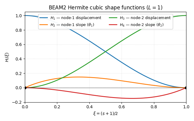
The 2-node 3D beam element (Euler-Bernoulli slender-beam limit) maps to the natural-coordinate segment \(s \in [-1, +1]\). Translations and torsion use linear shape functions; transverse displacement and slope use Hermite cubics so \(C^1\) continuity holds across element boundaries.

Linear shape functions (axial + torsion):

\[N_1^L(s) = \tfrac{1 - s}{2}, \qquad N_2^L(s) = \tfrac{1 + s}{2}.\]

Hermite cubic shape functions (transverse displacement and slope, mapped to the physical length \(L\)):

\[H_1(\xi) = 2\xi^{3} - 3\xi^{2} + 1, \quad H_2(\xi) = L\,(\xi^{3} - 2\xi^{2} + \xi),\]

\[H_3(\xi) = -2\xi^{3} + 3\xi^{2}, \quad H_4(\xi) = L\,(\xi^{3} - \xi^{2}),\]

with \(\xi = (s + 1)/2 \in [0, 1]\). H_1 and H_3 interpolate the two nodal displacements; H_2 and H_4 interpolate the two nodal slopes.

References

• Cook, R. D., Malkus, D. S., Plesha, M. E., Witt, R. J. (2002) Concepts and Applications of Finite Element Analysis, 4th ed., Wiley, §2.4–§2.6, Table 16.3-1.

• Zienkiewicz, O. C., Taylor, R. L. (2013) The Finite Element Method: Its Basis and Fundamentals, 7th ed., §2.5.1 eqs. (2.26)–(2.27).

• Przemieniecki, J. S. (1968) Theory of Matrix Structural Analysis, McGraw-Hill, §5.

Implementation: femorph_solver.elements.beam2.Beam2.

from __future__ import annotations

import matplotlib.pyplot as plt
import numpy as np
import pyvista as pv

Hermite cubic basis on [0, 1]

L = 1.0  # element length
xi = np.linspace(0.0, 1.0, 200)
H1 = 2.0 * xi**3 - 3.0 * xi**2 + 1.0
H2 = L * (xi**3 - 2.0 * xi**2 + xi)
H3 = -2.0 * xi**3 + 3.0 * xi**2
H4 = L * (xi**3 - xi**2)

fig, ax = plt.subplots(1, 1, figsize=(6.4, 4.0))
ax.plot(xi, H1, label="$H_1$ — node-1 displacement", color="#1f77b4", lw=2)
ax.plot(xi, H2, label="$H_2$ — node-1 slope ($\\theta_1$)", color="#ff7f0e", lw=2)
ax.plot(xi, H3, label="$H_3$ — node-2 displacement", color="#2ca02c", lw=2)
ax.plot(xi, H4, label="$H_4$ — node-2 slope ($\\theta_2$)", color="#d62728", lw=2)
ax.axhline(0.0, color="black", lw=0.5)
ax.axhline(1.0, color="grey", lw=0.5, ls=":")
ax.scatter([0.0, 1.0], [0.0, 0.0], color="black", zorder=5)
ax.set_xlabel(r"$\xi = (s + 1) / 2$")
ax.set_ylabel("$H_i(\\xi)$")
ax.set_title("BEAM2 Hermite cubic shape functions ($L = 1$)")
ax.legend(loc="upper center", ncol=2, fontsize=9, framealpha=0.95)
ax.set_xlim(0.0, 1.0)
ax.set_ylim(-0.2, 1.05)
ax.grid(True, ls=":", alpha=0.5)
fig.tight_layout()
fig.show()

Sanity — boundary conditions of the Hermite basis

The four Hermite cubics satisfy a Kronecker-delta-like property at the two endpoints \(\xi = 0\) (node 1) and \(\xi = 1\) (node 2):

	H1	H2	H3	H4
ξ=0 H’ ξ=1 H’	1 0 0 0	0 L 0 0	0 0 1 0	0 0 0 L

vals = np.array([[H1[0], H2[0], H3[0], H4[0]], [H1[-1], H2[-1], H3[-1], H4[-1]]])
np.testing.assert_allclose(vals[0], [1, 0, 0, 0], atol=1e-12)
np.testing.assert_allclose(vals[1], [0, 0, 1, 0], atol=1e-12)
print("OK — Hermite cubics interpolate displacements and slopes at the nodes.")

OK — Hermite cubics interpolate displacements and slopes at the nodes.

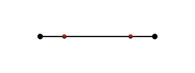
2-node beam reference (s ∈ [-1, +1])

cells = np.array([2, 0, 1])
cell_types = np.array([pv.CellType.LINE], dtype=np.uint8)
beam = pv.UnstructuredGrid(cells, cell_types, np.array([[-1.0, 0.0, 0.0], [+1.0, 0.0, 0.0]]))

# 2-point Gauss-Legendre on [-1, +1].
g = 1.0 / np.sqrt(3.0)
gauss = np.array([[-g, 0.0, 0.0], [+g, 0.0, 0.0]])

plotter = pv.Plotter(off_screen=True, window_size=(640, 240))
plotter.add_mesh(beam, color="black", line_width=4)
plotter.add_points(
    np.array([[-1.0, 0.0, 0.0], [+1.0, 0.0, 0.0]]),
    render_points_as_spheres=True,
    point_size=18,
    color="black",
    label="end nodes (2)",
)
plotter.add_points(
    gauss,
    render_points_as_spheres=True,
    point_size=14,
    color="#d62728",
    label="2-pt Gauss-Legendre",
)
plotter.view_xy()
plotter.camera.zoom(1.6)
plotter.show()