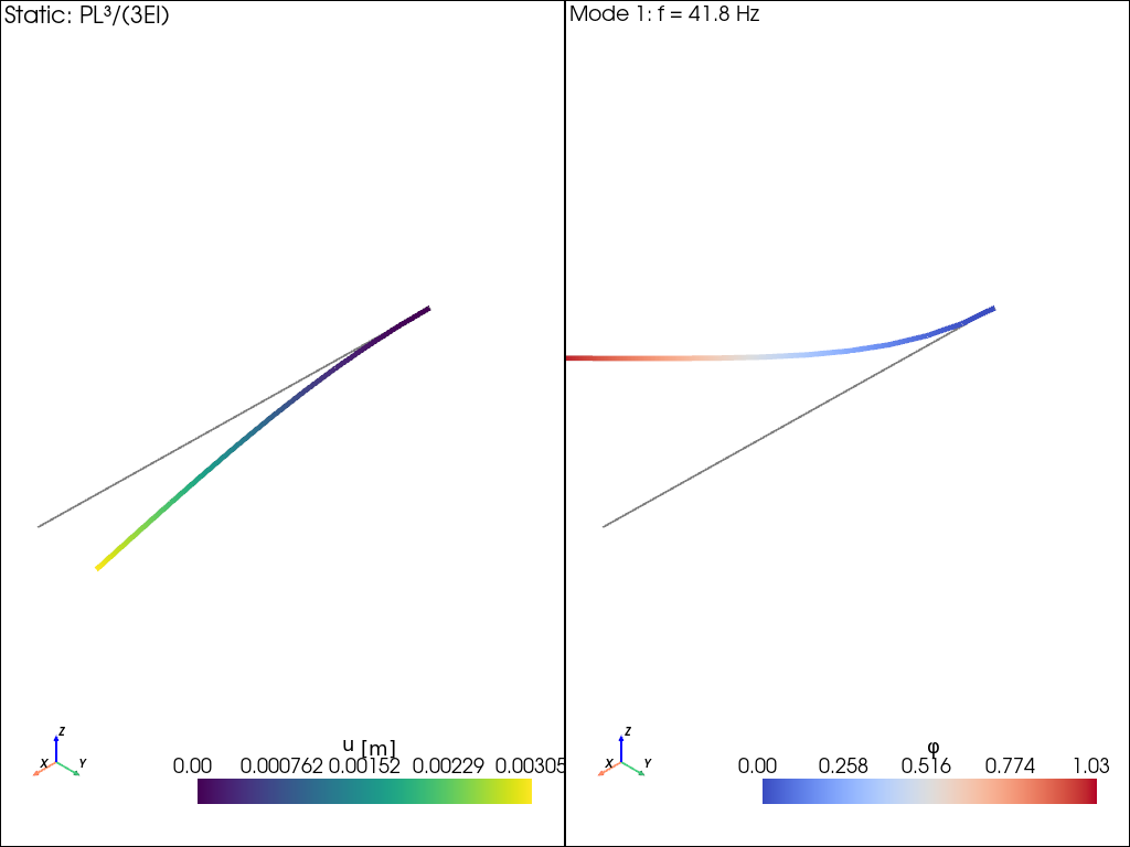
BEAM2 — cantilever tip deflection and first mode

Slender steel cantilever modelled with a line of BEAM2 elements. Two validations:

1. Static tip deflection matches P L³ / (3 E I) (Euler–Bernoulli).

2. First natural frequency matches (β₁ L)² √(E I / (ρ A L⁴)) with β₁ L = 1.87510407.

from __future__ import annotations

import numpy as np
import pyvista as pv
from vtkmodules.util.vtkConstants import VTK_LINE

import femorph_solver
from femorph_solver import ELEMENTS

Problem data

Steel, square 50 × 50 mm section, 1 m span, 1 kN tip load.

E = 2.1e11  # Pa
NU = 0.3
RHO = 7850.0  # kg/m³
b = 0.050  # m (square side)
A = b * b
I = b**4 / 12.0  # about either principal axis (square)
J = 2.0 * I  # thin-square torsion approximation
L = 1.0  # m
P = 1.0e3  # N (transverse tip load, +y)

N_ELEM = 10  # discretisation along the span

Build the model

BEAM2 has 6 DOFs per node; d(node, "ALL") on the clamped end fixes all six. Hermite-cubic shape functions recover Euler–Bernoulli exactly for prismatic beams, so 10 elements is already machine-precise on the static answer.

points = np.array(
    [[i * L / N_ELEM, 0.0, 0.0] for i in range(N_ELEM + 1)],
    dtype=np.float64,
)
cells_list: list[int] = []
for i in range(N_ELEM):
    cells_list.extend([2, i, i + 1])
cells = np.asarray(cells_list, dtype=np.int64)
cell_types = np.full(N_ELEM, VTK_LINE, dtype=np.uint8)
grid = pv.UnstructuredGrid(cells, cell_types, points)

m = femorph_solver.Model.from_grid(grid)
m.assign(
    ELEMENTS.BEAM2,
    material={"EX": E, "PRXY": NU, "DENS": RHO},
    real=(A, I, I, J),
)

m.fix(nodes=[1], dof="ALL")  # fully clamp node 1
m.apply_force(N_ELEM + 1, fy=P)  # tip load in +y

Static solve + analytical comparison

static = m.solve()
dof = m.dof_map()
tip_uy = np.where((dof[:, 0] == N_ELEM + 1) & (dof[:, 1] == 1))[0][0]
u_tip = static.displacement[tip_uy]
u_expected = P * L**3 / (3.0 * E * I)

print(f"BEAM2 tip UY       = {u_tip:.6e} m")
print(f"Analytical PL³/(3EI) = {u_expected:.6e} m")
assert np.isclose(u_tip, u_expected, rtol=1e-8)

BEAM2 tip UY       = 3.047619e-03 m
Analytical PL³/(3EI) = 3.047619e-03 m

Modal solve + analytical comparison

The transverse DOFs in two planes give two (degenerate) first bending modes. Because I_y = I_z here, femorph-solver’s eigensolver will return them both at the same frequency.

modal = m.modal_solve(n_modes=4)
BETA_L = 1.87510407  # dimensionless cantilever eigenvalue (first mode)
omega_expected = BETA_L**2 * np.sqrt(E * I / (RHO * A * L**4))
omega1 = float(np.sqrt(modal.omega_sq[0]))
omega2 = float(np.sqrt(modal.omega_sq[1]))

print(f"Expected ω₁  = {omega_expected:.4f} rad/s")
print(f"Computed ω₁  = {omega1:.4f} rad/s")
print(f"Computed ω₂  = {omega2:.4f} rad/s (bending in the other plane)")
assert np.isclose(omega1, omega_expected, rtol=5e-3)

Expected ω₁  = 262.4853 rad/s
Computed ω₁  = 262.4855 rad/s
Computed ω₂  = 262.4855 rad/s (bending in the other plane)

Plot the deflected shape and the first mode

Scatter the static displacement onto the grid for visualisation, then overlay the first mode shape coloured by transverse amplitude.

grid = m.grid.copy()
disp = np.zeros((grid.n_points, 3), dtype=np.float64)
mode_disp = np.zeros_like(disp)
for i, nn in enumerate(grid.point_data["ansys_node_num"]):
    rows = np.where(dof[:, 0] == int(nn))[0]
    for r in rows:
        d_idx = int(dof[r, 1])
        if d_idx < 3:  # translations only for warping
            disp[i, d_idx] = static.displacement[r]
            mode_disp[i, d_idx] = modal.mode_shapes[r, 0]

# Scale mode to unit peak
peak = float(np.max(np.abs(mode_disp))) or 1.0
mode_disp /= peak

grid.point_data["static_disp"] = disp
grid.point_data["mode1_disp"] = mode_disp

plotter = pv.Plotter(shape=(1, 2), off_screen=True)
plotter.subplot(0, 0)
plotter.add_text("Static: PL³/(3EI)", font_size=10)
plotter.add_mesh(grid, style="wireframe", color="gray", line_width=2)
plotter.add_mesh(
    grid.warp_by_vector("static_disp", factor=50.0),
    scalars=np.linalg.norm(disp, axis=1),
    line_width=5,
    scalar_bar_args={"title": "|u| [m]"},
)
plotter.add_axes()

plotter.subplot(0, 1)
plotter.add_text(f"Mode 1: f = {modal.frequency[0]:.1f} Hz", font_size=10)
plotter.add_mesh(grid, style="wireframe", color="gray", line_width=2)
plotter.add_mesh(
    grid.warp_by_vector("mode1_disp", factor=0.3),
    scalars=np.linalg.norm(mode_disp, axis=1),
    line_width=5,
    cmap="coolwarm",
    scalar_bar_args={"title": "|φ|"},
)
plotter.add_axes()
plotter.link_views()
plotter.show()