HEX8 — cantilever-plate modal (2 × 40 × 40 hex mesh)

End-to-end modal-analysis example: build a 1 m × 1 m × 10 mm steel plate as a 2-through-thickness, 40 × 40 in-plane hex mesh in pyvista, wrap it in femorph_solver.Model, clamp the x = 0 edge, and extract the first 10 modes with femorph_solver.Model.modal_solve().

from __future__ import annotations

import numpy as np
import pyvista as pv

import femorph_solver
from femorph_solver import ELEMENTS

Problem data

Steel, thin plate.

E = 2.0e11
NU = 0.3
RHO = 7850.0

LX, LY, LZ = 1.0, 1.0, 0.01
NX, NY, NZ = 40, 40, 2

Build the mesh in pyvista

StructuredGrid gives a regular block lattice; casting to UnstructuredGrid promotes every voxel to a VTK_HEXAHEDRON cell, which is exactly the HEX8 connectivity femorph-solver expects. No /PREP7 commands are replayed.

xs = np.linspace(0.0, LX, NX + 1)
ys = np.linspace(0.0, LY, NY + 1)
zs = np.linspace(0.0, LZ, NZ + 1)
xx, yy, zz = np.meshgrid(xs, ys, zs, indexing="ij")

grid = pv.StructuredGrid(xx, yy, zz).cast_to_unstructured_grid()
print(f"plate: {grid.n_points} nodes, {grid.n_cells} HEX8 cells")

plate: 5043 nodes, 3200 HEX8 cells

Wrap the grid as a femorph-solver model

Model.from_grid() auto-stamps sequential ids for nodes, elements, element-type, material, and real-constant when the grid doesn’t carry them. The caller only needs to declare et / mp.

m = femorph_solver.Model.from_grid(grid)
m.assign(ELEMENTS.HEX8, material={"EX": E, "PRXY": NU, "DENS": RHO})

Clamp the x=0 edge

All DOFs (UX, UY, UZ) fixed on every node with x ≈ 0.

node_coords = np.asarray(grid.points)
node_nums = np.asarray(grid.point_data["ansys_node_num"])
clamp_mask = node_coords[:, 0] < 1e-9
m.fix(nodes=node_nums[clamp_mask].tolist(), dof="ALL")
print(f"clamped {int(clamp_mask.sum())} nodes on x=0 edge")

clamped 123 nodes on x=0 edge

Modal solve

First 10 modes with the consistent mass matrix.

res = m.modal_solve(n_modes=10)

print("Mode     ω² [rad²/s²]          f [Hz]")
for i, (omsq, f) in enumerate(zip(res.omega_sq, res.frequency), start=1):
    print(f"{i:>3}   {omsq:>18.6e}   {f:>12.4f}")

Mode     ω² [rad²/s²]          f [Hz]
  1         8.806855e+03        14.9359
  2         2.473127e+04        25.0290
  3         3.449432e+05        93.4747
  4         4.237133e+05       103.5991
  5         4.648509e+05       108.5118
  6         1.190777e+06       173.6742
  7         2.719869e+06       262.4787
  8         2.833014e+06       267.8826
  9         3.009421e+06       276.0970
 10         4.123460e+06       323.1849

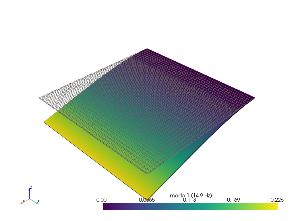
Plot the first mode shape

femorph_solver.io.modal_result_to_grid() attaches one (n_points, 3) displacement array and one magnitude scalar per mode to the grid, so plotting any mode is just warp_by_vector on mode_{k}_disp. Established commercial solvers (e.g. MAPDL POST1 PLDISP) emit the same per-mode shape data — this is the canonical post-processing flow.

grid_plot = femorph_solver.io.modal_result_to_grid(m, res)
phi1 = grid_plot.point_data["mode_1_disp"]

plotter = pv.Plotter(off_screen=True)
plotter.add_mesh(grid_plot, style="wireframe", color="gray")
plotter.add_mesh(
    grid_plot.warp_by_vector("mode_1_disp", factor=0.2 / np.max(np.abs(phi1))),
    scalars="mode_1_magnitude",
    show_edges=False,
    scalar_bar_args={"title": f"mode 1 ({res.frequency[0]:.1f} Hz)"},
)
plotter.add_axes()
plotter.show()

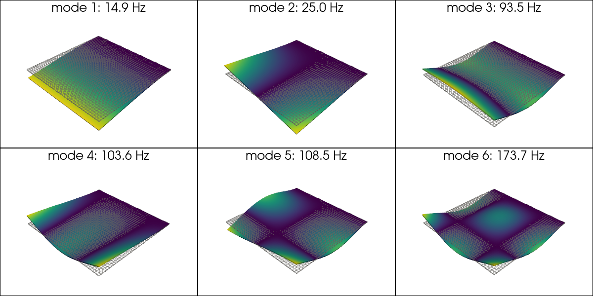
Plot the first six mode shapes as a 2 × 3 grid

Same grid carries all 10 modes, so a multi-viewport plotter can render any subset without a second modal solve. This is how every established post-processor users typically browse the mode spectrum in POST1.

plotter = pv.Plotter(shape=(2, 3), off_screen=True, window_size=(1200, 600))
for idx in range(6):
    row, col = divmod(idx, 3)
    plotter.subplot(row, col)
    phi_k = grid_plot.point_data[f"mode_{idx + 1}_disp"]
    factor = 0.1 / (np.max(np.abs(phi_k)) + 1e-300)
    plotter.add_mesh(grid_plot, style="wireframe", color="gray", opacity=0.35)
    plotter.add_mesh(
        grid_plot.warp_by_vector(f"mode_{idx + 1}_disp", factor=factor),
        scalars=f"mode_{idx + 1}_magnitude",
        show_edges=False,
        cmap="viridis",
        show_scalar_bar=False,
    )
    plotter.add_text(
        f"mode {idx + 1}: {res.frequency[idx]:.1f} Hz",
        position="upper_edge",
        font_size=10,
    )
plotter.show()