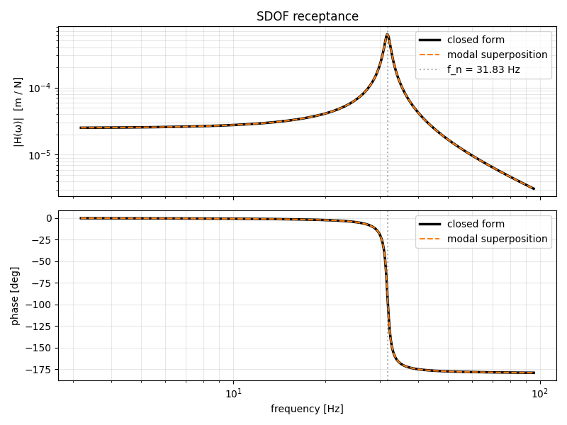
SDOF receptance — closed form vs modal superposition

A single-DOF mass-spring-damper has the analytical receptance

\[H(\omega) \;=\; \frac{1}{k - m\,\omega^{2} + i\,\omega\,c}\]

This example drives the same SDOF system through solve_harmonic_modal() and overlays the modal-superposition output on the closed form. With a single retained mode, the superposition reproduces the closed form to machine precision — the curves overlap exactly.

Tuning the example

• The eigenvalue ω_n = √(k / m) sets the resonance peak.

• The damping ratio ζ = c / (2 √(k m)) sets the height.

• Reducing damping makes the peak taller; the closed-form and modal curves still match.

References

• Ewins, D. J. Modal Testing: Theory, Practice and Application, 2nd ed., Research Studies Press (2000), §2.3 — receptance formulation used throughout this example.

• Craig, R. R. and Kurdila, A. J. Fundamentals of Structural Dynamics, 2nd ed., Wiley (2006), §11.4 — modal superposition for forced harmonic response.

from __future__ import annotations

import matplotlib.pyplot as plt
import numpy as np
import scipy.sparse as sp

from femorph_solver.solvers.harmonic import solve_harmonic_modal

1-DOF mass-spring-damper

m = 1.0  # kg
k = 4.0e4  # N/m → ω_n = 200 rad/s, f_n ≈ 31.83 Hz
zeta = 0.02
c = 2.0 * zeta * np.sqrt(k * m)

omega_n = np.sqrt(k / m)
f_n_hz = omega_n / (2.0 * np.pi)
print(f"Resonance: ω_n = {omega_n:.2f} rad/s   f_n = {f_n_hz:.3f} Hz   ζ = {zeta:.3f}")

K = sp.csr_array(np.array([[k]], dtype=np.float64))
M = sp.csr_array(np.array([[m]], dtype=np.float64))

Resonance: ω_n = 200.00 rad/s   f_n = 31.831 Hz   ζ = 0.020

Excitation sweep

Span 0.1 ω_n through 3 ω_n on a log grid so the resonance peak is well-resolved without piling samples at the high-frequency tail.

freq = np.geomspace(0.1 * f_n_hz, 3.0 * f_n_hz, 400)

Modal-superposition response

F = np.array([1.0], dtype=np.complex128)  # unit forcing on the single DOF
res = solve_harmonic_modal(
    K,
    M,
    F,
    frequencies=freq,
    n_modes=1,
    modal_damping_ratio=zeta,
)

Closed-form receptance

omega = 2.0 * np.pi * freq
H_closed = 1.0 / (k - m * omega**2 + 1j * omega * c)

# Sanity-check: with one retained mode the two should match to floating
# point precision.
np.testing.assert_allclose(res.displacement[:, 0], H_closed, atol=1e-12, rtol=1e-12)
print(
    "Modal-superposition matches closed form to "
    f"max |Δ| = {np.max(np.abs(res.displacement[:, 0] - H_closed)):.2e}"
)

Modal-superposition matches closed form to max |Δ| = 0.00e+00

Overlay the magnitude / phase

fig, (ax_mag, ax_phase) = plt.subplots(2, 1, sharex=True, figsize=(8, 6))

ax_mag.loglog(freq, np.abs(H_closed), "k-", lw=2.5, label="closed form")
ax_mag.loglog(freq, np.abs(res.displacement[:, 0]), "C1--", lw=1.5, label="modal superposition")
ax_mag.axvline(f_n_hz, color="grey", linestyle=":", alpha=0.6, label=f"f_n = {f_n_hz:.2f} Hz")
ax_mag.set_ylabel("|H(ω)|  [m / N]")
ax_mag.set_title("SDOF receptance")
ax_mag.grid(True, which="both", alpha=0.3)
ax_mag.legend()

phase = np.angle(res.displacement[:, 0], deg=True)
phase_closed = np.angle(H_closed, deg=True)
ax_phase.semilogx(freq, phase_closed, "k-", lw=2.5, label="closed form")
ax_phase.semilogx(freq, phase, "C1--", lw=1.5, label="modal superposition")
ax_phase.axvline(f_n_hz, color="grey", linestyle=":", alpha=0.6)
ax_phase.set_xlabel("frequency [Hz]")
ax_phase.set_ylabel("phase [deg]")
ax_phase.grid(True, which="both", alpha=0.3)
ax_phase.legend()

fig.tight_layout()
plt.show()