Full-rotor mode-shape slides via CyclicModel

Drives the bundled bladed-rotor sector through the CyclicModel API end-to-end:

1. Wrap the sector as a CyclicModel.

2. Call modal_solve() once — one CyclicModalResult per harmonic index \(k = 0 \ldots N/2\).

3. Expand each base-sector mode shape to the full rotor via femorph_solver.result._cyclic_expand.expand_mesh() and expand_mode_shape() — turn one sector’s complex eigenvector into N rotated real-valued snapshots that tile the full 360° rotor.

4. Lay the lowest non-rigid mode of every harmonic out as a subplot grid — one panel per \(k\), all rendered on the same full-rotor mesh so the wave structure is immediate.

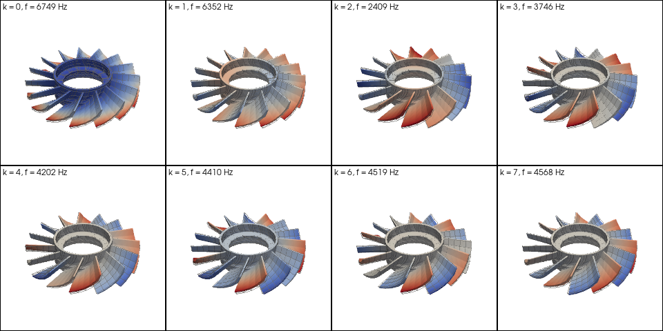
The “slide-show” framing comes from the spatial replication: every panel is the same instant in time, but each harmonic’s mode shape has a different number of nodal diameters around the circumference. Engine-order excitation analysis picks the harmonic whose nodal-diameter count matches the forcing pattern.

References

• Thomas, D. L. (1979) “Dynamics of rotationally periodic structures,” J. Sound Vib. 66 (4), 585–597.

• Wildheim, S. J. (1979) “Excitation of rotationally periodic structures,” J. Appl. Mech. 46, 891–893.

• Bathe, K.-J. (2014) Finite Element Procedures, 2nd ed., §10.3.4 (cyclic-symmetry modal).

from __future__ import annotations

import numpy as np
import pyvista as pv

import femorph_solver as fs
from femorph_solver.result._cyclic_expand import (
    expand_mesh,
    expand_mode_shape,
)

Load the bundled bladed-rotor sector

cyclic_bladed_rotor_sector_path() ships a 230-node, 101-cell HEX8 sector with the element-type / material / unit-system bookkeeping already stamped on the grid — ready for an immediate cyclic modal solve.

cm = fs.CyclicModel.from_pv(
    fs.examples.cyclic_bladed_rotor_sector_path(),
    n_sectors=15,
)
print(f"sector mesh: {cm.grid.n_points} nodes, {cm.grid.n_cells} cells")
print(f"full rotor : {cm.n_sectors * cm.grid.n_points} nodes")

sector mesh: 230 nodes, 101 cells
full rotor : 3450 nodes

Solve every harmonic index

A single CyclicModel.modal_solve() call returns one result per harmonic k = 0, 1, …, N // 2; for N = 15 that’s 8 indices (0 plus 1–7 — odd N has no Nyquist counter-rotating partner).

results = cm.modal_solve(n_modes=4)
print()
print(f"{'k':>3}  {'f_min(elastic) [Hz]':>22}")
for r in results:
    f = np.asarray(r.frequency, dtype=np.float64)
    elastic = f[f > 1.0]
    f_min = float(elastic[0]) if elastic.size else float("nan")
    print(f"{r.harmonic_index:>3}  {f_min:22.2f}")

k     f_min(elastic) [Hz]
0                 6748.95
1                 6352.36
2                 2408.67
3                 3746.20
4                 4202.18
5                 4410.26
6                 4519.15
7                 4567.99

Expand each sector to the full rotor mesh

The cyclic axis comes from the model itself (cm.axis); the axis-pivot point is the origin for this sector.

axis_dir = cm.axis
axis_point = np.zeros(3, dtype=np.float64)
full_grid = expand_mesh(cm.grid, n_sectors=cm.n_sectors, axis_point=axis_point, axis_dir=axis_dir)
print(f"expanded full-rotor mesh: {full_grid.n_points} nodes, {full_grid.n_cells} cells")

expanded full-rotor mesh: 3450 nodes, 1515 cells

Render the mode-shape slide grid

One subplot per harmonic k — each panel shows that harmonic’s lowest non-rigid mode warped onto the full rotor. The travelling-wave pair at harmonic k produces a pattern with k nodal diameters around the circumference; the rendering below makes that count visible without reading off frequencies.

def lowest_elastic_index(freq: np.ndarray, floor_hz: float = 1.0) -> int:
    """Index of the first non-rigid mode in a frequency vector."""
    elastic = np.where(np.asarray(freq, dtype=np.float64) > floor_hz)[0]
    return int(elastic[0]) if elastic.size else 0


nrows = 2
ncols = (len(results) + nrows - 1) // nrows
plotter = pv.Plotter(shape=(nrows, ncols), off_screen=True, window_size=(960, 480))

for panel_idx, r in enumerate(results):
    row, col = divmod(panel_idx, ncols)
    plotter.subplot(row, col)

    j = lowest_elastic_index(r.frequency)
    base_phi = np.asarray(r.mode_shapes)[:, j].reshape(-1, 3)

    # Expand the (complex) base sector across all N sectors at the
    # selected harmonic index — produces (N · n_base, 3) real-valued.
    full_phi = expand_mode_shape(
        base_phi,
        k=int(r.harmonic_index),
        n_sectors=cm.n_sectors,
        axis_dir=axis_dir,
    )
    amp = float(np.max(np.abs(full_phi))) or 1.0
    warp_factor = 0.05 / amp
    warped = full_grid.copy()
    warped.points = full_grid.points + warp_factor * full_phi
    warped["uz"] = full_phi[:, 2]

    plotter.add_text(
        f"k = {r.harmonic_index}, f = {float(np.asarray(r.frequency)[j]):.0f} Hz",
        font_size=9,
    )
    plotter.add_mesh(full_grid, style="wireframe", color="grey", opacity=0.3)
    plotter.add_mesh(warped, scalars="uz", cmap="coolwarm", show_edges=False, show_scalar_bar=False)

plotter.link_views()
plotter.view_isometric()
plotter.show()